
7. Likelihood Ratio and Score Processes#
Authors: Lars Peter Hansen (University of Chicago) and Thomas J. Sargent (NYU)
\(\newcommand{\eqdef}{\stackrel{\text{def}}{=}}\)
7.1. Introduction#
In this chapter we study the behavior of likelihood ratio processes and score processes. We treat these as processes so that we can study their dynamic behavior when additional observations are included. We start by showing how what we call multiplicative martingales imply alternative probability models. We then investigate some limiting behavior that reveals which among multiple models generates the data without imposing an ex ante distribution (a prior) over the alternative models. We then provide examples of such martingales constructed from likelihood ratio processes for alternative models. We end by studying the behavior of score processes that are constructed by differentiating log-likelihood with respect to an underlying parameter vector.
7.2. Multiplicative martingales#
Let \(\{ M_t : t \ge 0\}\) denote a process whose logarithm evolves as:
Thus the logarithmic counterpart is recognizable as an additive functional as studied in Chapter 4. We call such an \(\{ M_t : t \ge 0\}\) a multiplicative functional. We explore properties of such processes in some generality in Chapter 8. In this chapter, the processes of interest are multiplicative martingales:
Definition 7.1
The process \(M\) is a multiplicative martingale if
and thus \(E\left(M_{t+1} \mid M_t, X_t \right) = M_t.\)
Multiplicative martingales provide a convenient way to construct alternative probabilities.
Proposition 7.1
Suppose that \(\{ M_t : t \ge 0 \}\) is a multiplicative martingale. The ratio \(M_{t+1}/M_t\) implies a transition probability conditioned on \(X_t\) via the formula:
The resulting process for \(X\) remains Markovian, and the implied \(\tau\)-period transition probability can be represented as:
Proof. The linear operator:
maps nonnegative functions into nonnegative functions and the unit function into itself. Thus this operator is a conditional expectation. Moreover, it maps functions of \((w,x)\) into functions of \(x\) alone. This implies that \(\{X_t : t \ge 0\}\) is a first-order Markov process under the implied change of probability. The representation of the implied \(\tau\)-period conditional expectation operator follows from the Law of Iterated Expectations.
Remark 7.1
Under the change of measure induced by \(M_{t+1}/M_t\), the shock \(W_{t+1}\) typically does not have conditional mean zero.
So far we have not restricted the initial condition \(M_0\). We have only characterized its stochastic evolution. Suppose that the process \(\{X_t \}\) is stationary with probability denoted \(Q\), and consider \(M_0 = \tilde q(X_0)\) where \(\tilde q\) satisfies:
for all bounded (measurable) functions \(f\) of the Markov state \(x\). Then \({\widetilde Q}(dx) \eqdef {\tilde q}(x) Q(dx)\) is a stationary distribution under the probability measure that \(M\) implies.
In what follows we will impose such an initial condition on \(M_0\) in order that we can apply a Law of Large Numbers as characterized in Chapter 1. In addition we will impose the ergodic restriction that the only solutions to the equation:
are constant functions with \({\widetilde Q}\) measure one as investigated in Chapter 2.
7.3. Multiple models#
So far, we have considered two models, an initial one and a second one implied by a multiplicative martingale. Now suppose we have \(\ell + 1\) such models, comprising an initial one and \(\ell \) multiplicative martingales. We denote each such martingale as \(\{M^i_t : t \ge 0\}\) where each one induces a process that is stationary and ergodic. We may view the initial probability specification as one in which \(M^0_t = 1\) for all \(t\ge 0\). This is the ergodic decomposition of Chapter 1. Partition the sample space into \(\ell + 1\) invariant events, one matched to each martingale. Each martingale supplies the probabilities conditioned on its own event, and those conditional probabilities are what Definition 1.6 calls a statistical model. Distinguishing among the \(\ell+1\) models is therefore the problem of learning which invariant event occurred.
In this construction, we choose to normalize model zero to be the probability distribution used for representing all of the probabilities in conjunction with multiplicative martingales. Suppose instead we had used model one for this purpose. The \(\{M^i_t : t \ge 0\}\) processes cease to be martingales because we have changed the underlying probability. Instead, the ratio processes \(\{ M_t^i/M_t^1 : t \ge 0 \}\) are multiplicative martingales with this change in the underlying probabilities. This outcome of altering the baseline probability will be central in the discussion that follows.
7.4. Some large sample properties#
We next consider two gradient inequalities that we will use prominently. The function \(m\log m\) is convex and the function \(\log m\) is concave. A convex function lies above its gradient approximation and a concave function below its gradient approximation. Observe that the gradient is one for both functions when \(m=1\) and the gradient approximation is \(m-1\). Fig. 7.1 illustrates these two inequalities.
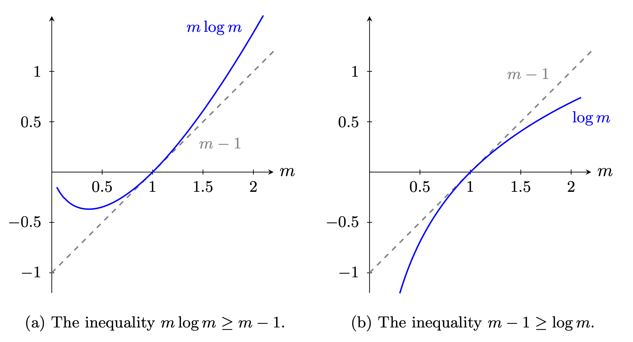
Fig. 7.1 Gradient inequalities#
We use these inequalities in conjunction with conditional expectations to obtain the targets of interest. This amounts to application of what is called Jensen’s Inequality and implies
These weak inequalities become strict when \(\log M_{t+1} - \log M_t\) is not equal to zero with probability one. Observe that \(\{ \log M_t : t \ge 0\}\) is an additive functional of the type studied in Chapter 4 with a trend coefficient that is negative. A consequence of the Law of Large Numbers and the first inequality in (7.1) is that:
Suppose now we consider expectations under the probabilities implied by the multiplicative martingale \(\{M_t : t \ge 0\}\). Then the second inequality in (7.1) implies that
These two limits give a large sample justification for use of the criterion
to determine which of the two models generates the data since the inequalities are strict when the multiplicative martingale is not degenerate.
Proposition 7.2
The process \(\{ \log M_t : t\ge 0\}\) is a supermartingale. That is,
The process \(\{ M_t \log M_t : t\ge 0 \}\) is a submartingale. That is,
These insights extend directly to the case of multiple models captured by alternative multiplicative martingales. It leads to the use of
as a way to select models with a large sample justification. As we will show, this approach has a direct application to the method of maximum likelihood.
We conclude this section by pointing to an unusual sample path property of multiplicative martingales.
Proposition 7.3
For a nondegenerate multiplicative martingale, \(\{M_{t} : t \ge 0 \}\) converges almost surely to zero even though \(E\left( \frac{M_{t}}{M_0} \mid X_0 \right) = 1\) for each \(t\).
Proof. We observed that by the Law of Large Numbers:
converges to a negative limit almost surely. This in turn implies that
almost surely.
[Martin, 2012] uses this type of result to argue that cumulative returns on long-dated assets that are positive martingales necessarily have distributions with fat tails. Section Illustrating the decompositions: a worked example of Chapter 8 quantifies this behavior for a log-normal example.
Here are some examples of multiplicative martingales constructed from some standard probability models.
Example 7.1
Consider a baseline Markov process having transition probability density \(\pi_o\) with respect to a measure \(\lambda\) over the state space \(\mathcal{X}\)
Let \(\pi\) denote some other transition density that we represent as
where we assume that \(\pi_o(x^+ \mid x) = 0\) implies that \(\pi(x^+ \mid x) = 0\) for all \(x^+\) and \(x\) in \(\mathcal{X}\).
Construct the multiplicative increment process as:
Example 7.2
Let an alternative model for a vector \(X\) be a vector autoregression:
where \({\mathbb A}\) is a stable matrix, \(\{W_{t+1} : t \ge 0 \}\) is an i.i.d. sequence of \({\cal N}(0,I)\) random vectors conditioned on \(X_0,\) and \({\mathbb B}\) is a square, nonsingular matrix. Assume that a baseline model for \(X\) has the same functional form but different settings \(({\mathbb A}_o, {\mathbb B}_o)\) of its parameters. Construct \(N_{t+1}\) as the one-period conditional log-likelihood ratio
Notice how the matrices \(({\mathbb A}_o, {\mathbb B}_o)\) of the baseline model and parameters \(({\mathbb A}, {\mathbb B})\) of the alternative model both appear.
Remark 7.2
Because \(\mathbb{B}\) is a nonsingular square matrix, model Example 7.2 has the same number of shocks, i.e., entries of \(W\), as there are components of \(X\). A more general setting would be a hidden Markov state model like the one presented in Section Kalman Filter and Smoother of Chapter 6 that has a time-invariant representation with an “information state vector” constructed as a way to condition on an infinite past of an observation vector.
7.5. Log likelihoods#
We now construct the function \(\kappa\) as the increment to a log-likelihood ratio. We let \(\theta\) denote a parameter vector, and suppose that a vector of date \(t+1\) observations \(Z_{t+1}\) is given by
Form:
where \(\psi(z^* \mid x, \theta)\) is the density of \(Z_{t+1}\) given \(X_{t}\) and \(\theta\). We further assume that given \((x, \theta)\), \(Z_{t+1}\) is informationally equivalent to \(W_{t+1}.\) This can be justified by an assumption that we can invert \(\phi\) as a function of \(W_{t+1}\). We assume that given \(\theta,\) \(X_t\) is revealed by past \(Z_t\) and possibly a finite number of lags. Model \(\theta_0\) is the baseline used for computing expectations.
By factoring a joint density we obtain a log-likelihood process conditioned on \((X_0, \theta)\) as:
Chapter 6 writes \(L_t(\theta)\) for the likelihood itself; here and in what follows \(L_t(\theta)\) is its logarithm. We apply our previous arguments to justify finding the
for a discrete set of models.[1] In what follows, we suppose there is a continuum of models.
7.6. Score processes#
In this section, we study first-order necessary conditions associated with the maximum likelihood estimator. For simplicity suppose that the parameter space \(\Theta\) is an open interval of \(\mathbb{R}\) containing the parameter value \(\theta_0\). Inequality (7.1) implies that the parameter value \(\theta_0\) necessarily maximizes the population objective
Importantly, this objective conditions on \(x\) and \(\theta_0\). Suppose that we can differentiate under the integral sign in (7.2) to get the first-order condition
Definition 7.2
The score process \(\{S_{t} : t = 0,1,\ldots \}\) is defined as
Theorem 7.1
\(E \left(S_{t+1} - S_t \mid X_t \right) = 0\), so the score process is an additive martingale with increment \(\frac{d}{d \theta} \log \psi(Z_j|X_{j-1}, \theta_0)\) under the \(\theta_0\) probability model. From the analysis in Chapter 3 and [Billingsley, 1961], we obtain a central limit approximation:
where \(V = E \left( \left[ \frac{d}{d \theta} \log \psi(Z_{t+1} |X_t, \theta_0)\right]^2 \right)\).
Proof. This follows directly from equation (7.3) and Proposition 3.2.
Theorem 7.1 justifies using the martingale central limit theorem Proposition 3.2 to characterize the large sample behavior of the score process. The resulting central limit approximation yields a large sample characterization of the maximum likelihood estimator of \(\theta\) in a Markov setting. With additional regularity conditions, the following result is typical:
where \(\theta_t\) maximizes the log likelihood function \(L_t(\theta)\). This kind of result motivates interpreting the covariance of the martingale increment of the score process
as a measure of the information in the data about the parameter \(\theta_0\). The scalar \(V\) is a measure of what is called Fisher information after the statistician R.A. Fisher. This analysis has a direct extension to the case where \(\theta\) is a vector.
Consider extending the notion of Fisher information to the following situation. There is a vector \(\theta\) of unknown parameters. We want a measure of information about one component of the parameter vector, although to get that information we have to estimate other components too. Call the first block the ‘parameters of interest’ and write \(\theta\) for it; call the second block the ‘nuisance parameters’ and write \(\vartheta\) for it. Suppose that the likelihood is parameterized on an open set \(\Theta\) in a finite dimensional Euclidean space and that the true parameter vector is \((\theta_0, \vartheta_0) \in \Theta\). Write the multivariate score process as
where \(\{ S_{t+1} : t=0,1,\ldots\}\) is the partial derivative of the log-likelihood with respect to \(\theta\) and \(\{ \tilde{S}_{t+1} : t=0,1,\ldots \}\) is the partial derivative with respect to \(\vartheta\). Estimating \(\vartheta_0\) simultaneously with \(\theta_0\) is more difficult than estimating \(\theta_0\) when knowing \(\vartheta_0\). Fisher’s measure of information corrects for the additional challenge of estimating \(\vartheta_0\) simultaneously in order to make inferences about \(\theta_0\). In particular, Fisher’s measure of information about \(\theta\) is the inverse of the \((1,1)\) component of the inverse of the covariance matrix \({\mathbb V}\), partitioned conformably with \(\theta, \vartheta\):
To represent this inverse in a revealing way, compute the population regression
where \(\beta\) is the population regression coefficient and \(U_{t+1}\) is the population regression residual that by construction is orthogonal to the regressor \((\tilde{S}_{t+1} - \tilde{S}_t)\). The population regression induces the representation
where \({\mathbb O}\) is a vector of zeros. Since \(U_{t+1}\) is orthogonal to \(\tilde{S}_{t+1} - \tilde{S}_t,\)
The inverse matrix is:
This equation reveals that the \((1,1)\) component of the partition of matrix \({\mathbb V}^{-1}\) is
We therefore take the Fisher information about \(\theta\) to be \(E(U_{t+1}^2)\), the reciprocal of \({\mathbb V}^{-1}_{1,1}\). By least squares theory, this measure satisfies
This inequality asserts that the likelihood function contains more information about \(\theta\) when \(\vartheta\) is known to be \(\vartheta_0\) than when \(\theta\) and \(\vartheta\) are both unknown.
Inequality (7.4) offers reasons to be cautious when ignoring the joint estimation challenge and pretending you know \(\vartheta\). This latter practice leads you to overstate the information in the sample about the parameter \(\theta\) of interest. Note that since the multivariate score \(\begin{bmatrix} S_{t+1} \\ \tilde{S}_{t+1} \end{bmatrix}\) is a vector of additive martingales, the score regression residual \(U_{t+1}\) is a martingale difference, so its partial sums form an additive martingale.
7.7. Using a multiplicative martingale for model selection#
We now return to the single multiplicative martingale as a way to model an alternative probability. Suppose we use the martingale at time \(t\), \(M_t,\) to construct a criterion for choosing between models. One choice is to check whether \(M_t\) is greater than or less than one for a sample of size \(t\). When \(M_t\) exceeds one, we choose the probability model induced by the multiplicative martingale. For motivation, recall from Proposition 7.3 that the martingale converges almost surely to zero. Thus the probability of exceeding a fixed threshold must decline to zero under the baseline specification. To provide a more refined result, we study probabilities of making mistakes when using this criterion. We follow [Chernoff, 1952] and others by applying what is called large deviation theory to study the probability of making a mistake if the baseline model used to represent expectations governs the data generation. We show how to characterize this probability for large sample sizes.
For notational convenience, we initialize \(M_0 = 1\) and condition on the date zero state \(X_0\). Should the \(\{M_t : t \ge 0\}\) of interest be initialized differently, in what follows we would use \(M_t/M_0\) and include \(M_0\) in the date zero conditioning information. Instead of carrying along the extra notation, we just change how we normalize the martingale. We construct a bound on the mistake probability by using an inequality that is implied by two facts:
The probability that \(M_t\) exceeds one is the expectation of the indicator function:
For a scalar \(\alpha > 0,\)
The left panel of Fig. 7.2 illustrates this inequality. Values of \(0 < \alpha < 1\) are of particular interest in which case \(m^\alpha\) is a concave increasing function. Thus we use the inequality
The expectation on the right side of this relation is more tractable to analyze than the one on the left side when we investigate behavior as \(t \rightarrow \infty.\) Since the inequality applies for arbitrary \(\alpha\), to produce approximations that are as sharp as possible, we will minimize over the choice of \(\alpha\).
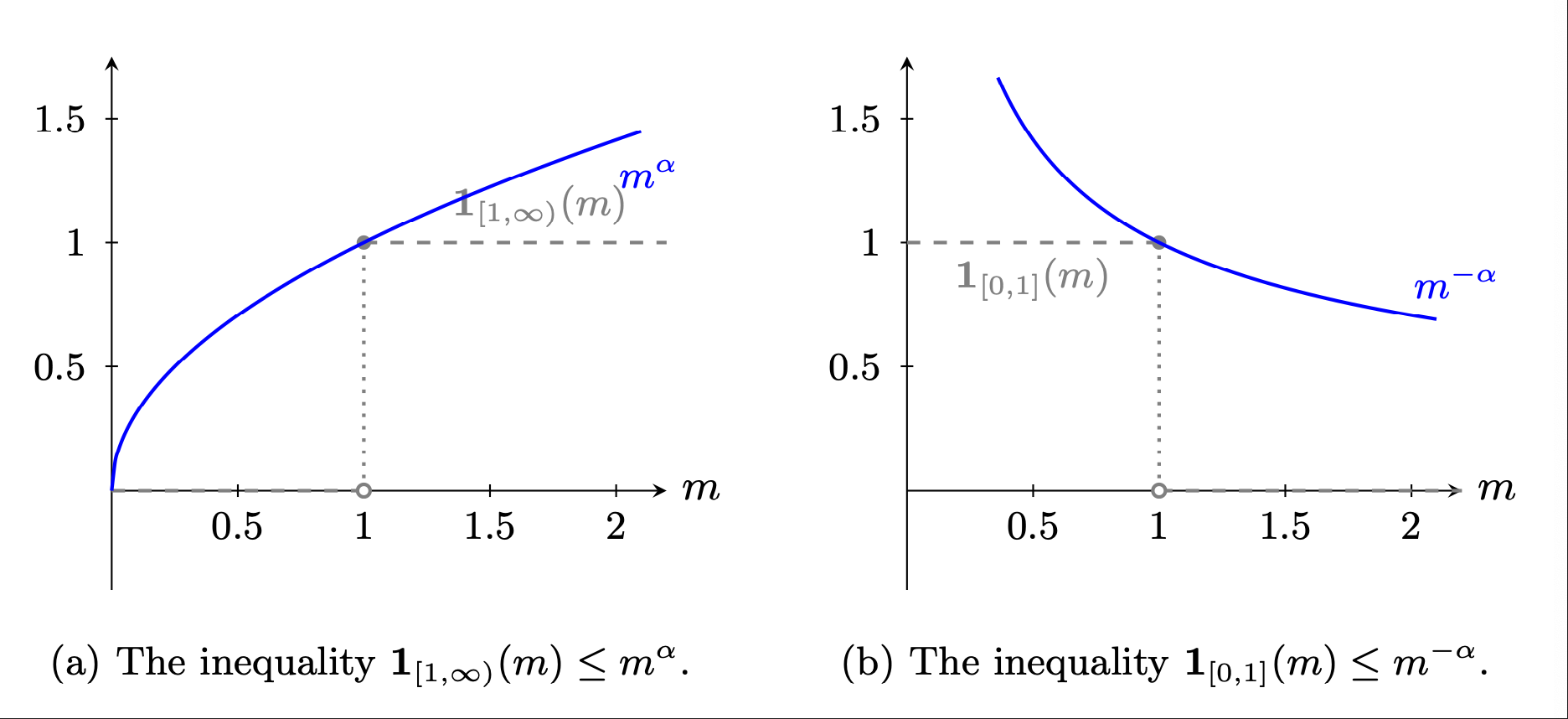
Fig. 7.2 Two indicator function inequalities with \(\alpha = \frac{1}{2}\).#
Note that \(m^\alpha\) for \(0 < \alpha < 1\) is a concave function. From the associated gradient inequality, the process \(\{ (M_t)^\alpha : t \ge 0 \}\) is a supermartingale. This uses the same logic as we used when showing that \(\{ \log M_t : t\ge 0\}\) is a supermartingale. The limit of interest is
The resulting \(\eta(\alpha)\) is interpretable as an asymptotic decay rate for the process \(\{(M_t)^\alpha : t \ge 0\}\). To obtain a sharp bound on the limiting behavior of the mistake probability we solve
Then \(\eta^*\) tells us the asymptotic decay rate in the probability of choosing the multiplicative martingale-based model when the original baseline model actually generates the data.
So far, we have only analyzed one type of mistake. The other possibility is that the alternative model with probabilities induced by the multiplicative martingale generates the data, and \(M_t < 1.\) In this case, the indicator function and the dominating function are given by:
as is illustrated in the right panel of Fig. 7.2. Since we are interested in computations under the alternative probability measure, we are led to study
Again, we maximize over \(\alpha\) and note that
The asymptotic decay rates of the two mistakes are equated when one is used as the threshold. The resulting decay rate is called Chernoff entropy. This finding does not imply that the two mistake probabilities are equated. But the rate equalization extends to constant thresholds other than one, including a Bayesian procedure with prior probabilities assigned to each model. Alternative constant thresholds will change the probabilities but not the asymptotic decay rates. Commonly employed classical methods that hold fixed one of the error probabilities independent of sample size do not have fixed thresholds and thus are not covered by this analysis. Nor are they well justified. In contrast to this common approach, fixed threshold rules have both mistake probabilities decay as more data become available.
In Chapter 8, we develop methods that, among other things, show how to compute the asymptotic decay rates.
Remark 7.3
Consider a Bayesian decision maker selecting a model. Let \(\pi_0\) denote the prior probability that the baseline model generates the data, and let \(\pi_m\) denote the prior probability that the alternative model implied by the multiplicative martingale generates the data. Let \(\upsilon_0\) denote the utility reward if the baseline model is chosen correctly, and let \(\upsilon_m\) denote the utility reward if the multiplicative martingale model is chosen correctly. At time \(t,\) the decision maker will select the baseline model by checking if the utility-weighted posterior probability of the baseline model exceeds the multiplicative model counterpart:
With a straightforward computation, this inequality simplifies to:
which is a constant threshold rule of the type we have been considering.
7.8. Summary#
A multiplicative martingale induces an alternative probability specification, and a likelihood ratio process is such a martingale. That is what allows a family of competing models to be represented as a family of martingales over a common baseline. The logarithm of each is an additive functional in the sense of Chapter 4 with a negative trend coefficient, which is why Proposition 7.3 holds: data eventually discriminate among the models without any prior over them. Chernoff entropy measures how fast.
Score processes come from differentiating a log likelihood with respect to a parameter, and are additive martingales. Their long-run variance is the Fisher information that limits what can be learned about the parameter, and inequality (7.4) records what is lost when nuisance parameters are unknown. Chapter 8 studies multiplicative functionals without imposing the martingale restriction, and Chapter 13 turns to estimation when no likelihood is specified at all.
7.9. Exercises#
Exercise 7.1 (A Gaussian likelihood ratio and its Chernoff entropy)
Model \(0\) asserts that a scalar observation \(Z_t\) is drawn i.i.d. from \({\mathcal N}(\mu_0, \sigma^2)\) and model \(1\) asserts that it is drawn i.i.d. from \({\mathcal N}(\mu_1, \sigma^2)\), with \(\mu_0 \ne \mu_1\) and \(\sigma^2 > 0\) known. Define the log-likelihood ratio increment
and the cumulated ratio \(\log M_t = \sum_{\tau=1}^t \kappa(Z_\tau)\), and write \(\delta = (\mu_1 - \mu_0)/\sigma\) for the signal-to-noise ratio.
(a) Show that \(\kappa(Z_{t+1}) = \frac{\mu_1 - \mu_0}{\sigma^2}Z_{t+1} - \frac{\mu_1^2 - \mu_0^2}{2\sigma^2}\), and that under model \(0\) it is distributed \({\mathcal N}\left(-\frac{\delta^2}{2}, \delta^2\right)\).
(b) Verify directly that \(\{M_t\}\) is a multiplicative martingale under model \(0\) in the sense of Definition 7.1, and confirm both inequalities of (7.1).
(c) Compute the asymptotic decay rate \(\eta(\alpha)\) for \(\alpha \in (0,1)\), find the maximizing \(\alpha^*\), and report the Chernoff entropy \(\eta^*\). Verify the symmetry \(\eta(1-\alpha) = \eta(\alpha)\) asserted in the chapter.
(d) How does \(\eta^*\) depend on \(\delta\), and what happens as \(\mu_1 \rightarrow \mu_0\)? Use Remark 7.3 to say what a Bayesian who assigns prior probabilities \(\pi_0, \pi_m\) would do differently, and whether it changes \(\eta^*\).
Exercise 7.2 (Fisher information in the presence of a nuisance parameter)
Take the same i.i.d. Gaussian setting, but now treat the parameters as unknown. The single-observation log-likelihood is
and the true values are \(\mu_0 = 0\), \(\sigma_0^2 = 1\).
(a) Compute the score increment \(\frac{d}{d\mu}\log \psi\left(Z_t \mid \mu_0\right)\) holding \(\sigma^2\) known, and verify that its expectation under the true model is zero, confirming (7.3).
(b) Compute the Fisher information \(V\) from the score, then verify the information equality by computing \(-{\mathbb E}_0\left[\frac{d^2}{d\mu^2}\log\psi\left(Z_t \mid 0\right)\right]\) and confirming that both give the same value.
(c) Now let \(\vartheta = \sigma^2\) be an unknown nuisance parameter alongside the parameter of interest \(\theta = \mu\). Compute the \(2 \times 2\) matrix \({\mathbb V}\), obtain the population regression coefficient \(\beta\) of the score for \(\mu\) on the score for \(\sigma^2\), and compute the residual variance \({\mathbb E}\left(U_{t+1}^2\right)\).
(d) Does inequality (7.4) hold strictly here? Explain which feature of the Gaussian family accounts for this, and give an informal argument for why the inequality would be strict in a family whose mean and variance share a parameter.
Exercise 7.3 (A likelihood ratio for two autoregressive models)
Consider two models for a scalar observation,
where \(W_{t+1}\) is a scalar standard normal shock, \({\sf f}_0, {\sf f}_1 > 0\), and \(X_t\) consists of \(Z_t\) and finitely many lags. Each model specifies coefficients \(\theta_j = \left({\sf n}_j, {\sf d}_j, {\sf f}_j\right)\) with \(\theta_1 \ne \theta_0\). Suppose model \(\theta_0\) generates the data.
(a) Use the date \(t+1\) contribution to the log-likelihood ratio of model \(1\) relative to model \(0\) to form \(\kappa(X_t, W_{t+1})\), and show that it can be written as \({\sf a}_t + {\sf b}_t W_{t+1} + {\frac {{\sf c}} 2}W_{t+1}^2\). Identify \({\sf a}_t\), \({\sf b}_t\), and \({\sf c}\), and note which of them depend on \(X_t\).
(b) Verify that \({\mathbb E}\left(\exp\left[\kappa(X_t, W_{t+1})\right] \mid X_t, \theta_0\right) = 1\), so the multiplicative functional is a martingale.
(c) Verify that \({\mathbb E}\left(\kappa(X_t, W_{t+1}) \mid X_t, \theta_0\right) < 0\), and identify the two separate sources of the strict inequality: one from the conditional means differing, one from the volatilities differing.
(d) Show that for \(0 < \alpha < 1\), \({\mathbb E}\left(\exp\left[\alpha \kappa(X_t, W_{t+1})\right] \mid X_t, \theta_0\right) < 1\), and state the restriction on \({\sf f}_0/{\sf f}_1\) needed for the expectation to be finite.
In checking these relations you may use the following. If \(W\) is standard normal then
for \({\sf c} < 1\). You do not have to derive it, although a complete-the-square argument does the job.
Exercise 7.4 (Computing a Chernoff entropy)
Continue with Exercise 7.3, but now suppose \({\sf d}_0 = {\sf d}_1 = 0\), so that \(X_t\) drops out of your formulas and the observations are i.i.d. Chapter 8 develops general methods for computing decay rates; this special case can be done by hand.
(a) Form \(\eta(\alpha) = -\log {\mathbb E}\left(\exp\left[\alpha\kappa\right] \mid \theta_0\right)\) as an explicit function of \(\alpha\) and maximize over \(0 < \alpha < 1\). You may do the maximization analytically, or numerically for a few parameter configurations.
(b) Specialize to \({\sf f}_0 = {\sf f}_1 = {\sf f}\). Show that \(\alpha^* = {\frac 1 2}\) and that the Chernoff entropy reduces to \(\left({\sf n}_0 - {\sf n}_1\right)^2/\left(8{\sf f}^2\right)\), recovering Exercise 7.1.
(c) Discuss the effect of raising \({\sf f}_0\) and \({\sf f}_1\) together while holding \({\sf n}_0\) and \({\sf n}_1\) fixed, and then of widening the gap between \({\sf n}_0\) and \({\sf n}_1\) while holding \({\sf f}_0 = {\sf f}_1\).
(d) Now let \({\sf f}_0 \ne {\sf f}_1\) with \({\sf n}_0 = {\sf n}_1\), so the models differ only in volatility. Show that the Chernoff entropy is still strictly positive, and that \(\alpha^* \ne {\frac 1 2}\) in general. What does the asymmetry of \(\eta(\cdot)\) about \({\frac 1 2}\) tell you that the equal-volatility case conceals?
7.10. Answers#
Solution to Exercise 7.1 (A Gaussian likelihood ratio and its Chernoff entropy)
(a) The \(\sigma^2\) terms cancel in the ratio, leaving
Writing \(Z_{t+1} = \mu_0 + \sigma W_{t+1}\) under model \(0\) and collecting terms,
which is \({\mathcal N}\left(-\delta^2/2, \delta^2\right)\).
(b) By the log-normal formula, \({\mathbb E}_0\left[\exp \kappa\right] = \exp\left(-\frac{\delta^2}{2} + \frac{\delta^2}{2}\right) = 1\), which is Definition 7.1. For (7.1), \({\mathbb E}_0(\kappa) = -\delta^2/2 < 0\) confirms the first inequality. For the second, under the alternative measure \(\kappa\) has mean \(+\delta^2/2\), since tilting by \(M\) shifts the mean of \(W\) from \(0\) to \(\delta\); so \({\mathbb E}_0\left[\kappa \exp \kappa\right] = {\widetilde{\mathbb E}}(\kappa) = +\delta^2/2 > 0\). The two inequalities are strict, as they must be whenever \(\delta \ne 0\).
(c) Since the \(\kappa\)’s are i.i.d.,
so
a downward parabola. Setting \(\eta'(\alpha) = (1-2\alpha)\delta^2/2 = 0\) gives \(\alpha^* = {\frac 1 2}\) and
Symmetry is immediate from the formula: \(\eta(1-\alpha) = \frac{(1-\alpha)\alpha \delta^2}{2} = \eta(\alpha)\). This is the concrete instance of the general claim in the chapter that the two mistake probabilities decay at a common rate.
(d) \(\eta^*\) grows with the squared signal-to-noise ratio. As \(\mu_1 \rightarrow \mu_0\) it goes to zero: the models become statistically indistinguishable, and the number of observations needed to separate them grows without bound. Small belief distortions can therefore survive statistical scrutiny, a theme taken up in Chapter 8.
By Remark 7.3, a Bayesian with priors \(\pi_0, \pi_m\) and utility rewards \(\upsilon_0, \upsilon_m\) compares \(M_t\) to the constant threshold \(\frac{\upsilon_0 \pi_0}{\upsilon_m\pi_m}\) rather than to one. Changing the threshold changes both mistake probabilities in finite samples, but not their exponential decay rates: a constant shifts \(\log M_t\) by a fixed amount while \(\log M_t\) itself drifts linearly in \(t\). So \(\eta^*\) is unchanged. The chapter’s warning applies here: a classical procedure that holds one error probability fixed as the sample grows does not use a fixed threshold and is not covered by this analysis.
Solution to Exercise 7.2 (Fisher information in the presence of a nuisance parameter)
(a) With \(\sigma^2 = 1\), \(\frac{d}{d\mu}\log\psi(Z_t\mid\mu) = Z_t - \mu\), which at \(\mu_0 = 0\) is \(Z_t\). Under the true model \({\mathbb E}(Z_t) = 0\), confirming (7.3).
(b) From the score, \(V = {\mathbb E}\left(Z_t^2\right) = 1\). From the second derivative, \(\frac{d^2}{d\mu^2}\log\psi = -1\), so \(-{\mathbb E}_0\left[\frac{d^2}{d\mu^2}\log\psi\right] = 1\). Both give \(V = 1\).
(c) The two score increments at \(\left(\mu_0,\sigma_0^2\right) = (0,1)\) are
Under \({\mathcal N}(0,1)\) we have \({\mathbb E}Z^2 = 1\), \({\mathbb E}Z^4 = 3\), and all odd moments vanish. Hence
so
The off-diagonal zero gives \(\beta = 0\), hence \(U_{t+1} = Z_{t+1}\) and \({\mathbb E}\left(U_{t+1}^2\right) = 1 = {\mathbb E}\left[\left(S_{t+1}-S_t\right)^2\right]\).
(d) No: (7.4) holds with equality. The responsible feature is that the two scores are orthogonal, which for the Gaussian family is the population counterpart of the independence of the sample mean and the sample variance. Not knowing \(\sigma^2\) costs nothing when the object of interest is \(\mu\).
The Fisher information about \(\theta\) is the squared length of the component of the \(\theta\)-score orthogonal to the \(\vartheta\)-score. Whenever the two scores are correlated, that projection strictly shortens the vector and the inequality is strict. Suppose instead that a single parameter governed both moments, say \(Z_t \sim {\mathcal N}\left(\theta, \theta^2\right)\). Then perturbing \(\theta\) moves the mean and the spread together, a change in location can be partly mimicked by a change in scale, and the two directions of the likelihood surface are no longer orthogonal. The data can then say less about location alone than they could if the scale were known, the caution the chapter attaches to inequality (7.4).
Solution to Exercise 7.3 (A likelihood ratio for two autoregressive models)
(a) The conditional density of \(Z_{t+1}\) given \(X_t\) under model \(j\) is normal with mean \({\sf n}_j + \left({\sf d}_j\right)^\top X_t\) and variance \({\sf f}_j^2\). Under model \(0\) the realized observation satisfies \(Z_{t+1} - {\sf n}_0 - \left({\sf d}_0\right)^\top X_t = {\sf f}_0 W_{t+1}\), so
Therefore
which is of the stated form with
Only \({\sf a}_t\) and \({\sf b}_t\) depend on the state, and they do so only through \({\sf m}_t\), the gap between the two conditional means. The quadratic coefficient \({\sf c}\) is a constant reflecting the volatility discrepancy alone.
(b) Here \(1 - {\sf c} = {\sf f}_0^2/{\sf f}_1^2 > 0\), so the formula applies:
The two \({\sf m}_t^2\) terms cancel, which makes the ratio a martingale for every state.
(c) Since \({\mathbb E}W = 0\) and \({\mathbb E}W^2 = 1\), \({\mathbb E}\left[\kappa\mid X_t\right] = {\sf a}_t + {\sf c}/2\). Writing \({\sf r} = {\sf f}_0^2/{\sf f}_1^2\),
Both terms are non-positive. The first vanishes only at \({\sf r} = 1\), by strict concavity of the logarithm at \(1\); it is the contribution of the volatility discrepancy. The second vanishes only when \({\sf m}_t = 0\); it is the contribution of the conditional mean discrepancy. Two models can therefore be distinguished either because they disagree about where \(Z_{t+1}\) will be or because they disagree about how uncertain it is, and the log-likelihood drifts down under either kind of disagreement.
(d) Applying the formula with \(\alpha \kappa = \alpha{\sf a}_t + \alpha{\sf b}_t W + \frac{\alpha{\sf c}}{2}W^2\),
which is finite provided \(\alpha {\sf c} < 1\). Since \({\sf c} = 1 - {\sf f}_0^2/{\sf f}_1^2 < 1\) always, and \(\alpha \in (0,1)\), the requirement \(\alpha {\sf c} < 1\) is automatic. That the expectation is strictly less than one is the gradient inequality of the chapter: \(m^\alpha\) is strictly concave on \((0,\infty)\) for \(\alpha \in (0,1)\), so by Jensen’s inequality \({\mathbb E}\left[\left(e^{\kappa}\right)^\alpha\right] < \left({\mathbb E}\left[e^\kappa\right]\right)^\alpha = 1\), using (b). This is the inequality that underlies the fixed-threshold analysis of the chapter and delivers a strictly positive decay rate.
Solution to Exercise 7.4 (Computing a Chernoff entropy)
(a) With \({\sf d}_0 = {\sf d}_1 = 0\), \({\sf m}_t = {\sf m} \eqdef {\sf n}_0 - {\sf n}_1\) is constant, so \({\sf a}\) and \({\sf b}\) no longer depend on the state and the \(\kappa\)’s are i.i.d. Taking the negative logarithm of the expression in part (d) of Exercise 7.3,
with \({\sf a}, {\sf b}, {\sf c}\) as before. Chernoff entropy is \(\eta^* = \max_{0<\alpha<1}\eta(\alpha)\), which is a one-dimensional concave maximization easily done numerically.
(b) If \({\sf f}_0 = {\sf f}_1 = {\sf f}\) then \({\sf c} = 0\), \({\sf a} = -{\sf m}^2/\left(2{\sf f}^2\right)\), and \({\sf b} = -{\sf m}/{\sf f}\). The logarithmic term drops and
the same parabola as in Exercise 7.1 with \(\delta\) replaced by \({\sf m}/{\sf f}\). So \(\alpha^* = {\frac 1 2}\) and
(c) Raising \({\sf f}_0 = {\sf f}_1 = {\sf f}\) with the means fixed lowers \(\eta^*\) like \(1/{\sf f}^2\): noisier data make the two models harder to tell apart, and the decay rate of both mistake probabilities falls. Widening \(\left|{\sf n}_0 - {\sf n}_1\right|\) with \({\sf f}\) fixed raises \(\eta^*\) quadratically: the models make increasingly different predictions and a moderate sample suffices. Only the ratio \({\sf m}/{\sf f}\) matters, not its two ingredients separately.
(d) With \({\sf n}_0 = {\sf n}_1\) we have \({\sf m} = 0\), hence \({\sf b} = 0\) and \({\sf a} = \log\left({\sf f}_0/{\sf f}_1\right)\), so
This is strictly positive on \((0,1)\) whenever \({\sf f}_0 \ne {\sf f}_1\), so models differing only in volatility are still statistically distinguishable, and at an exponential rate. Differentiating, the maximizer solves \(\frac{{\sf c}}{2\left(1-\alpha{\sf c}\right)} = -\log\frac{{\sf f}_0}{{\sf f}_1}\), whose solution is not \({\frac 1 2}\) except in the degenerate case \({\sf f}_0 = {\sf f}_1\).
In the equal-volatility case \(\eta(\cdot)\) is symmetric about \({\frac 1 2}\) because the two models are equally far from each other: the roles of numerator and denominator in the likelihood ratio can be exchanged without changing anything. When volatilities differ, that exchange symmetry is broken. A high-volatility model assigns non-negligible probability to data a low-volatility model regards as nearly impossible, but not the reverse, so evidence accumulates asymmetrically. Chernoff entropy remains a single number equalizing the two decay rates, as the chapter shows, but it is now attained at an \(\alpha^*\) tilted toward one of the models, and that tilt is the quantitative record of the asymmetry.