2. Markov Processes

Download PDF here

Authors: Lars Peter Hansen (University of Chicago) and Thomas J. Sargent (NYU)

\(\newcommand{\eqdef}{\stackrel{\text{def}}{=}}\)

2.1. Introduction

Chapter 1 defined random vectors to be functions that map sample points into vectors of real numbers. To construct a stochastic process that describes probabilistic fluctuations over time, we used a transformation that maps sample points into sample points in conjunction with a probability measure over sample points. This approach reveals the version of the Law of Large Numbers pertinent for time series analysis with the associated nuances. We used this formulation to construct what we called a statistical model as well as probabilities over alternative statistical models. In practice, this approach is not the typical starting point for applied research. When researchers want to specify a stochastic process, they directly specify a joint distribution over a sequence of random vectors. In Chapter 1 we produced these as “induced distributions.” Importantly, we showed how to work backwards by specifying a collection of joint distributions in a temporally consistent way to build a probability measure on a canonical space. We then use this canonical construction to verify key constructs such as measure-preserving, stationarity, invariant events, and ergodic building blocks from Chapter 1.

This chapter starts with a widely used way of specifying probabilities over infinite sequences well-known as a Markov process. The task in this chapter is to investigate how to establish the various key constructs of the previous chapter, providing a convenient way to apply the seemingly abstract constructs we investigated previously.

In Markov process theory, we call a random vector, \(X_t,\) the state because it probabilistically specifies the position of a dynamic system at time \(t\) from the perspective of a model builder or an econometrician. We construct a consistent sequence of probability distributions \(Pr_\ell\) for a sequence of random vectors

\[\begin{split}X^{[\ell]} \doteq \begin{bmatrix} X_0 \\ X_1 \\ \vdots \\ X_\ell \end{bmatrix}\end{split}\]

for all nonnegative integers \(\ell\) by specifying the two elementary components of a Markov process: (i) a probability distribution for \(X_0\), and (ii) a time-invariant distribution for \(X_{t+1}\) conditional on \(X_t\) for \(t \geq 0\). The vector \(X_t\) suffices for conditioning on the entire history of the process. The joint probabilities for \(X_{t+j}\) for \(j \geq 0\) can be built from these two distributions. By creatively defining the state vector \(X_t\), many models used in applied research can be cast as a Markov process.

2.2. Constituents

Assume a state space \(\mathcal{X}\) and a transition distribution \(P(dx^*|x)\). For example, \(\mathcal{X}\) could be \(\mathbb{R}^n\) or a subset of \(\mathbb{R}^n\). The transition distribution \(P\) is a conditional probability measure for each \(X_t = x\) in the state space. The conditional probability measure \(P(dx^* |x)\) assigns probabilities to next period’s state given that this period’s state is \(x\). Since it is a conditional probability measure, it satisfies

\[\int_{\{x^* \in \mathcal{X} \}}P(dx^* | x) = 1\]

for every \(x\) in the state space. Thus, integration is over \(x^*\) and conditioning is captured by \(x\), where \(x^*\) is a possible realization of next period’s state and \(x\) is a realization of this period’s state.

In addition, once we specify an initial distribution \(Q_0\) for the initial state vector \(X_0\) over \(\mathcal{X}\), then we have completely specified all joint distributions for the stochastic process \(\{X_t : t = 0, 1, \ldots\}\).

Often, though not always, the conditional distributions have densities with respect to a common distribution \(\lambda(dx^*)\) to be used to integrate over states. That lets us use a transition density to represent the conditional probability measure:

\[P(dx^* | x) = p(x^* | x) \lambda(dx^*)\]

where the conditional densities with respect to the measure \(\lambda\) satisfy:

\[\int_{\{x^* \in \mathcal{X} \}} p(x^* | x ) \lambda(dx^*) = 1\]

for every \(x\) in the state space.

Example 2.1

A first-order vector autoregression is a Markov process. Consider \(m\) such processes, indexed by \(i\). The index \(i\) represents a discrete form of parameter uncertainty. We can include \(i\) as an additional time-invariant component of the state. Here \(P(dx^*|x, i )\) is a normal distribution with mean \({\mathbb A}_ix\) and covariance matrix \({\mathbb B}_i{{\mathbb B}_i}'\) for square matrices \({\mathbb A}_i\) and matrices \({\mathbb B}_i\) with full column rank.[1] These assumptions imply a vector autoregressive representation (VAR) for \(i=1,2,..., m.\)

\[Y_{t+1} = {\mathbb A}_i Y_t + {\mathbb B}_i W_{t+1} ,\]

for \(t \geq 0\), where \(W_{t+1}\) is a multivariate standard normally distributed random vector that is independent of \(Y_t, i\).

Here we have specified a collection of Markov processes. We can express this collection as a single first-order Markov process with an augmented state \(x= (y,i)\). The evolution of the second component of the state vector would be viewed as an invariant random variable, making it a degenerate component of the composite Markov process. That second component could be initialized at any of the \(m\) parameter configurations. The invariance follows from \(i\) being a model that does not change over time.

Example 2.2

To construct a discrete-state Markov chain, suppose that \(\mathcal{X}\) consists of \(n\) possible states. We can label these states in a variety of ways, but for mathematical convenience, suppose that state \(x_j\) is the coordinate vector consisting entirely of zeros except in position \(j\), where there is a \(1\). Represent \(Q_0\) as a vector \(q\) of probabilities for each of the states, and represent the transition probabilities as a matrix \({\mathbb P} = [p_{ij}]\) with one row and one column for each possible value of the state \(x\). Entry \((i,j)\) is the probability of moving from state \(i\) to state \(j\) in a single period.

It is useful to construct an operator by applying a one-step conditional expectation operator to functions of a Markov state. Let \(f:{\mathcal X} \rightarrow {\mathbb R}\). For bounded \(f\), define:

(2.1)\[{\mathbb T} f (x) = E \left[ f(X_{t+1}) | X_t = x \right] = \int_{\{x^* \in {\mathcal X}\}} f(x^*) P(d x^*|x).\]

The Law of Iterated Expectations justifies iterating on \({\mathbb T}\) to form conditional expectations of the function \(f\) of the Markov state over longer horizons:

\[{\mathbb T}^j f(x) = E \left[ f(X_{t+j}) | X_t = x \right].\]

As an alternative approach for modeling a Markov process, we begin with an operator \({\mathbb T}\) appropriately restricted as follows. Indeed, by applying \({\mathbb T}\) to a suitable range of ``test functions,’’ \(f\), we can construct a conditional probability measure, \(P(dx^* | x)\).

Theorem 2.1

Let \({\mathbb T}\) be a linear operator that maps a space of (Borel measurable) bounded functions into itself. We can use \({\mathbb T}\) to construct a conditional probability measure \(P(dx^*|x)\) provided that \({\mathbb T}\) is (a) well-defined on the space of bounded functions, (b) preserves the bound, (c) maps nonnegative functions into nonnegative functions, and (d) maps the unit function into the unit function.

Example 2.2 (cont’d)

We can use Example 2.2 to illustrate the preceding theorem. We can represent the conditional expectation operator by using the transition matrix \({\mathbb P}.\) Think of a function of the Markov state as an \(n\)-dimensional vector with each coordinate giving the value of the function at the respective coordinate. Thus, we use a vector \(\textbf{f}\) to represent a function from the state space to the real line. Each coordinate of \(\textbf{f}\) gives the value of the function at the corresponding coordinate vector. Then the conditional expectation operator \(\mathbb{T}\) can be represented in terms of the transition matrix \(\mathbb{P}\):

\[E(\textbf{f} \cdot X_{t+1} | X_t = x) = \mathbb{T}\textbf{f} \cdot x = x'\mathbb{P} \textbf{f}.\]

Conditional expectations are obtained by applying the matrix \({\mathbb P}\) to vectors that depict functions of interest. Alternatively, we might begin with a matrix representation of the conditional expectations \(\mathbb{T} \textbf{f}\) for alternative \(n\)-dimensional vectors \(\textbf{f}\) where the entries of \(\mathbb{T}\) are nonnegative. Moreover, suppose applying \({\mathbb T}\) to \({\mathbb 1}_n\), a vector of ones, satisfies the eigenvalue problem:

\[{\mathbb T}{\mathbb 1}_n = {\mathbb 1}_n.\]

Observe that applying \({\mathbb T}\) to alternative coordinate vectors recovers transition probabilities. In this example, the conditional expectation operator of interest is represented with the matrix of transition probabilities: \({\mathbb T} = {\mathbb P}\).

In what follows it will sometimes be convenient to represent a Markov process with a conditional expectation operator that embeds the transition probabilities. As we have seen, it is straightforward to go back and forth between the transition probabilities and the one-period conditional expectation.

2.3. Stationarity

We can construct a stationary Markov process by carefully choosing the distribution of the initial state \(X_0\).

Definition 2.1

A probability measure \(Q\) over a state space \(\mathcal{X}\) for a Markov process with transition probability \(P\) is a stationary distribution if it satisfies

\[\int_{ \{ x \in \mathcal{X} \}} P(d x^*|x) Q(dx) = Q(d x^*).\]

We will sometimes refer to a stationary density \(q\). A density is always relative to a measure. With this in mind, let \(\lambda\) be a measure used to integrate over possible Markov states on the state space \(\mathcal{X}\). Then a density \(q\) is a nonnegative (Borel measurable) function of the state for which \(\int q(x) \lambda(dx) = 1\).

Definition 2.2

A stationary density over a state space \(\mathcal{X}\) for a Markov process with transition probability \(P\) is a probability density \(q\) with respect to a measure \(\lambda\) over the state space \(\mathcal{X}\) that satisfies

\[\int P(d x^*|x) q(x) \lambda(dx) = q(x^*) \lambda(dx^*).\]

Example 2.2 (cont’d)

We again revisit Example 2.2. The stationary probabilities satisfy:

\[{\sf q}_j = \sum_{i=1}^n {\sf q}_i p_{ij}\]

where \({\sf q}_j\) is the probability of state \(j\) and \(p_{ij}\) is the probability of going from state \(i\) to state \(j\). Using the matrix representation for the transition probabilities, the vector, \({\textbf q}\), of stationary probabilities satisfies:

\[{\textbf q}' {\mathbb P} = {\textbf q}', \]

where the entries of \({\textbf q}\) are restricted to be nonnegative and sum to one. Thus the vector \({\textbf q}\) is a row eigenvector of the matrix \({\mathbb P}\).

Example 2.3

Various sufficient conditions imply the existence of a stationary distribution. Given a transition distribution \(P\), one such condition that is widely used to justify some calculations from numerical simulations is that the Markov process be time reversible, which means that

(2.2)\[P(dx^*|x) Q(dx) = P(dx|x^*) Q(dx^*)\]

for some probability distribution \(Q\) on \(\mathcal{X}\). Because a transition distribution satisfies \(\int_{\{ x \in \mathcal{X}\}} P(dx|x^*) =1 \),

\[\int_{\{ x \in \mathcal{X}\}} P(dx^*|x) Q(dx) = \int_{\{ x \in \mathcal{X}\}} P(dx|x^*) Q(dx^*) = Q(dx^*) ,\]

so \(Q\) is a stationary distribution by Definition 2.1. Restriction (2.2) implies that the process is time reversible in the sense that forward and backward transition distributions coincide. Time reversibility is special, so later we will explore other sufficient conditions for the existence of stationary distributions.[2]

Remark 2.1

When a Markov process starts at a stationary distribution, we can build the process \(\{ X_t : t=0,1,...\}\) with a measure-preserving transformation \({\mathbb S}\) of the type featured in Chapter 1, Section Representing a Stochastic Process using the canonical construction.

2.4. \({\mathcal L}^2,\) Eigenfunctions, and Invariant Events

We connected Laws of Large Numbers to a statistical notion of invariance in Chapter 1. The word invariance brings to mind a generalization of eigenvectors called eigenfunctions. Eigenfunctions of a linear mapping characterize an invariant subspace of functions such that the application of a linear mapping to any element of that space remains in the same subspace. Eigenfunctions associated with a unit eigenvalue are themselves invariant under the mapping. So perhaps it is not surprising that such eigenfunctions of \({\mathbb T}\) come in handy for characterizing invariant events implied by a Markov process.

2.4.1. Eigenfunctions with Unit Eigenvalues

A mathematically convenient space for our analysis uses a given stationary distribution \(Q\) to form the space of functions

\[{\mathcal L}^2 = \{ f:{\mathcal X} \rightarrow {\mathbb R} : \int f(x)^2 Q(dx) < \infty \} .\]

It can be verified that \({\mathbb T} : {\mathcal L}^2 \rightarrow {\mathcal L}^2\) and that

\[\| f \| = \left[\int f(x)^2 Q(dx)\right]^{1/2} \]

is a well-defined norm on \({\mathcal L}^2\).[3]

We now study eigenfunctions of the conditional expectation operator \({\mathbb T}\).

Definition 2.3

A function \(f \in \mathcal{L}^2\) that solves \(\mathbb{T} f = f\) is an eigenfunction of \(\mathbb{T}\) associated with a unit eigenvalue.

The following proposition asserts that an eigenfunction \({{\tilde f}}(X_t)\) associated with a unit eigenvalue is constant as \(X_t\) moves through time.

Proposition 2.1

Suppose that \({\tilde f}\) is an eigenfunction of \(\mathbb{T}\) associated with a unit eigenvalue. Then \(\{{\tilde f}(X_t) : t=0,1,...\}\) is constant over time with probability one.

Proof.

\[E \left[{\tilde f}(X_{t+1}) {\tilde f}(X_t)\right] = \int (\mathbb{T}{\tilde f})(x) {\tilde f}(x) Q(dx) = \int {\tilde f}(x)^2 Q(dx) = E \left[\tilde{f}(X_t)^2\right]\]

where the first equality follows from the Law of Iterated Expectations. Then because \(Q\) is a stationary distribution,

\[\begin{eqnarray*} E\left([{\tilde f}(X_{t+1}) - {\tilde f}(X_t)]^2\right) & = & E\left[{\tilde f}(X_{t+1})^2\right] + E \left[{\tilde f}(X_t)^2\right] \cr &&- 2 E\left[ {\tilde f}(X_{t+1}){\tilde f}(X_t) \right] \cr & = & 0. \end{eqnarray*}\]

From Proposition 2.1 we know that time-series averages formed using an eigenfunction \({\mathbb T} {\tilde f} = {\tilde f}\) are invariant over time, so

\[{\frac 1 N} \sum_{t=1}^N {\tilde f}(X_t) = \tilde f(X_0).\]

Thus this proposition verifies that we can use such eigenfunctions to study invariant events since the resulting stochastic processes are constant over time. However, when \( f(x)\) varies across sets of states \(x\) that occur with positive probability under \(Q\), a time series average \({\frac 1 N} \sum_{t=1}^N f(X_t)\) can differ from \(\int f(x) Q(dx)\). This happens when observations of \( f(X_t)\) along a sample path for \(\{X_t\}\) convey an inaccurate impression of how \(f(x)\) varies across the stationary distribution \(Q(dx)\).

2.4.2. Invariant events for a Markov process

In this section, we describe how to construct invariant events for a Markov process expressed in terms of subsets of the state space. We suggest how to construct such sets using eigenfunctions associated with unit eigenvalues.

Given one eigenfunction with a unit eigenvalue, we start by showing how to construct other ones. Let \({f}\) denote such an eigenfunction, and let \(\phi : {\mathbb R} \rightarrow {\mathbb R}\) be a bounded Borel measurable function. Since \(\{ {f}(X_t) : t=0,1,2,... \}\) is invariant over time, so is \(\left\{ \phi\left[{f}(X_t)\right] : t=0,1,2, \ldots \right\}\) and it is necessarily true that

\[{\mathbb T} (\phi \circ {f}) = \phi \circ {f}.\]

Therefore, from an eigenfunction \({f}\) associated with a unit eigenvalue, we can construct other eigenfunctions.[4] A class of examples of \(\phi\) that are particularly interesting are indicator functions expressed as:

(2.3)\[\begin{split}\phi[{f}(x)] = \begin{cases} 1 & \text{if} \ {f}(x) \in {\tilde {\mathfrak b}} \\ 0 & \text{if} \ {f}(x) \notin {\tilde {\mathfrak b}} \end{cases}\end{split}\]

for some Borel set \({\tilde {\mathfrak b}}\) in \({\mathbb R}\).

It follows that

\[\Lambda = \{ \omega \in \Omega : {f}[X_0(\omega)] \in {\tilde {\mathfrak b}} \}\]

is an invariant event in \(\Omega\). Note that by constructing the Borel set, \({\mathfrak b}\) in \(\mathcal X\)

\[{\mathfrak b} = \{ x : {f}(x) \in {\tilde {\mathfrak b}} \}\]

we can represent \(\Lambda\) as

(2.4)\[\Lambda = \{ \omega \in \Omega : X_0(\omega) \in {\mathfrak b} \}.\]

Thus we have shown how to construct many eigenfunctions, starting from an initial such function. This in turn gives us a way to construct invariant events represented by the initial \(X_0\) residing in subsets of the state space \({\mathcal X}.\) For Markov processes, all invariant events can be represented as in (2.4), which is expressed in terms of the initial state \(X_0\). See [Doob, 1953]. It then follows from our previous logic that indicator functions of invariant events are eigenfunctions of \({\mathbb T}\) with unit eigenvalues. This construction of invariant events is depicted in Fig. 2.1

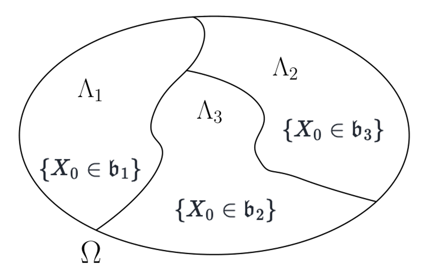
Fig. 2.1 To illustrate invariant event structure in a Markov environment, we plot a partition with three invariant events, \(\Lambda_1, \Lambda_2, \Lambda_3.\) Each of the events can be represented in terms of the initial state \(X_0\) as noted in the figure.

2.5. Ergodic Markov Processes

Chapter 1 studied special statistical models that, because they are ergodic, are affiliated with a Law of Large Numbers in which limit points are constant across sample points \(\omega \in \Omega\). Section Ergodic Decomposition described other statistical models that are not ergodic and that are components of more general probability specifications that we used to express the idea that a statistical model is unknown. As we described, even when the statistical model is unknown, ergodic processes remain of interest as they are building blocks (specific statistical models) that are revealed over time. We now investigate ergodicity in the context of Markov processes.

Proposition 2.2

When the only solutions to the equation

\[{\mathbb T}f = f\]

are constant functions (with \(Q\) measure one), then it is possible to construct \(\{ X_t : t=0,1,2,...\}\) as a stationary and ergodic Markov process with \({\mathbb T}\) as the one-period conditional expectation operator and \(Q\) as the initial distribution for \(X_0\).

Evidently, ergodicity is a property that obtains relative to a stationary distribution \(Q\) of the Markov process. If there are multiple stationary distributions, it is possible that there is a function \(f\) that is constant under one stationary probability distribution, \(Q,\) and ceases to be constant with probability one and still solves \({\mathbb T}f = f\) with other choices of a stationary distribution. All of this is consistent with our decomposition of measure-preserving probabilities discussed in Chapter 1. Our aim in this section is to provide an interpretable sufficient condition for constructing initial probabilities for a Markov process that imply an ergodic ``building block.’’

Suppose now we consider any Borel set \(\mathfrak{b}\) of \(\mathcal{X}\) that has \(Q\) measure that is neither zero nor one. Let \(f\) be constructed as the indicator function of the set \(\mathfrak{b}\) without restricting \(\mathfrak{b}\) to be an invariant event in \(\mathfrak{J}\). Then \(\mathbb{T}^j\) applied to \(f\) is the conditional probability of \(\left\{X_j \in \mathfrak{b}\right\}\) as of date zero. If we want time series averages to converge to unconditional expectations, we must require that the set \(\mathfrak{b}\) be visited eventually with positive probability. To account properly for all possible future dates, we use a mathematically convenient resolvent operator defined by

\[\mathbb{M} f(x)=(1-\lambda) \sum_{j=0}^{\infty} \lambda^j \mathbb{T}^j f(x).\]

for some constant discount factor \(0<\lambda<1\). As economists, we recognize \({\mathbb M}\) as a discounted conditional expectation as of date zero of current and future \(f(X_t)\)’s scaled by \(1-\lambda.\) This scaling converts the expected discounted value into a geometric average with weights \((1- \lambda) \lambda^j\) for \(j=0,1,\dots\).

Notice that if \(f\) is an eigenfunction of \(\mathbb{T}\) associated with a unit eigenvalue, then the same is true for \(\mathbb{T}^j\) and hence for \(\mathbb{M}\). Suppose that \(f\) is an indicator function for a set \(\mathfrak{b}\) with positive \(Q\) probability. The conditional expectations \(\mathbb{T}^j\) compute probabilities of the Markov process visiting \(\mathfrak{b}\) in future time periods given a current state \(x\). Applying \({\mathbb M}\) to this indicator function and asking that it be strictly positive gives a formal sense that the Markov process eventually visits the set \(\mathfrak{b}\). The following proposition extends this restriction to all nonnegative functions that are distinct from zero. This is sufficient for the Markov process to be ergodic.

Proposition 2.3

Suppose that for any \(f \ge 0\) such that \(\int f(x) Q(dx) > 0\), \({\mathbb M} f(x) > 0\) for all \(x \in {\mathcal X}\) with \(Q\) measure one. Then any solution \({f}\) to \({\mathbb T} f = f\) is necessarily constant with \(Q\) measure one.

Proof. Consider an eigenfunction \({\tilde f}\) associated with a unit eigenvalue. The function \(f = \phi \circ {\tilde f}\) necessarily satisfies:

\[{\mathbb M}f = f\]

for any \(\phi\) of the form (2.3). If such an \(f\) also satisfies \(\int f(x) Q(dx) > 0\), then \(f(x)=1\) with \(Q\) probability one. Since this holds for any Borel set \({\mathfrak b}\) in \({\mathbb R}\), \({f}\) must be constant with \(Q\) probability one.

Remark 2.2

Proposition 2.3 supplies a sufficient condition for ergodicity. A more restrictive sufficient condition is that there exists an integer \(m \geq 1\) such that

\[{\mathbb T}^{m} f(x) > 0\]

on a set with \(Q\) measure one, for any \(f \ge 0\) such that \(\int f(x) Q(dx) > 0.\)

Remark 2.3

The sufficient conditions imposed in Proposition 2.3 imply a property called irreducibility relative to the probability measure \(Q\). While this proposition presumes that \(Q\) is a stationary distribution, the concept of irreducibility allows for a more general specification of the measure \(Q\).

Definition 2.4

The process \(\{ X_t \}\) is said to be irreducible with respect to \(Q\) if for any \(f \ge 0\) such that \(\int f(x) Q(dx) > 0\), \({\mathbb{M}} f(x) > 0\) for all \(x \in {\mathcal{X}}\) with \(Q\) measure one.

We summarize our ergodic characterization by the following proposition.

Proposition 2.4

When \(Q\) is a stationary distribution and \(\left\{ X_t \right\}\) is irreducible with respect to \(Q\), the process is necessarily ergodic.

Proposition 2.4 provides a way to verify ergodicity.

2.6. Taking Inventory

We now take inventory of our analysis of Markov processes so far.

• From a specification of Markov transition probabilities, we can deduce stationary distributions \(Q\) over the Markov state that are preserved over time, as characterized by the equation in Definition 2.1. Multiple stationary distributions \(Q\) can satisfy instances of this equation. Such situations are of special interest to applied statisticians.

• Invariant events for a Markov process have a special structure described by (2.4). Here invariant events are represented in terms of an initial state \(X_0\).

• Instead of working directly with the transition probabilities, we can use an associated conditional expectation operator \({\mathbb T}\). Eigenfunctions with unit eigenvalues define invariant random variables. The Markov process is ergodic with respect to a particular stationary probability measure \(Q\) when all such eigenfunctions are constant with \(Q\) probability one.

• As an instructive alternative, we construct a resolvent operator \({\mathbb M}\) that is a geometrically weighted average of the \({\mathbb T}^j\)’s, for \(j \ge 0\). The Markov process is ergodic if, for any nonnegative \(f\) that has strictly positive expectation computed using a particular stationary distribution \(Q\), \({\mathbb M}f\) is strictly positive with \(Q\) measure one.

• Chapter 1 presented ergodicity as a property of a statistical model. As applied statisticians, we sometimes entertain a set of Markov models, each of which is ergodic. Here ergodicity can be checked by using either of the two approaches just described. Associated with each such possible model is a stationary distribution. We can regard these as building-block \(Q\)’s and can take the associated ergodic Markov models as constituents of a specification to be used in an empirical application. It is possible that there is a finite number of these building blocks, a countable number, or even a continuum of them that is indexed by an unknown parameter vector.

• The smallest convex set containing all building-block \(Q\)’s (the convex hull) forms a collection of stationary probabilities for the Markov process.

2.7. Periodicity

Next, we study a notion of periodicity of a stationary and ergodic Markov process.[5] To define periodicity of a Markov process, for a given positive integer \(p\) we construct a new Markov process by sampling an original process every \(p\) time periods. This is sometimes called ‘skip-sampling’ at sampling interval \(p\).[6] With a view toward applying Proposition 2.1 to \({\mathbb T}^p\), solve

(2.5)\[{\mathbb T}^p f = f\]

for a function \({f}\). We know from Proposition 2.1 that for an \(f\) that solves (2.5), \(\{ {f}(X_t) : t=0, p, 2p, \ldots \}\) is invariant and so is \(\{ {f}(X_t) : t=1,p+1,2p+1,...\}\). The process \({f}(X_t)\) is periodic with period \(p\) or \(np\) for any positive integer \(n\).

Definition 2.5

The periodicity of an irreducible Markov process \(\left\{ X_t \right\}\) with respect to \({Q}\) is the smallest positive integer \(p\) such that there is a solution to equation (2.5) that is not constant with \({ Q}\) measure one. When there is no such integer \(p\), we say that the process is aperiodic.

Theorem 2.2

Consider a counterpart of the resolvent operator \({\mathbb M}\) constructed by sampling at an interval given by positive integer \(p\):

(2.6)\[{\mathbb M}_p f(x) = (1 - \lambda) \sum_{j=0}^\infty \lambda^{j} {\mathbb T}^{pj} f.\]

Provided that \({\mathbb M}_p f(x) > 0\) with \({Q}\) measure one and all \(p \ge 0\) for any \(f \ge 0\) such that \(\int f(x) Q(dx) > 0\), the Markov process is aperiodic.

2.8. Finite-State Markov Chains

We reconsider Example 2.2 where \(\mathcal{X}\) consists of \(n\) possible states. We use a vector \(\textbf{f}\) to represent a function from the state space to the real line. Each coordinate of \(\textbf{f}\) gives the value of the function at the corresponding coordinate vector. Recall that the conditional expectation operator \(\mathbb{T}\) can be represented in terms of the transition matrix \(\mathbb{P}\):

\[E(\textbf{f} \cdot X_{t+1} | X_t = x) = (\mathbb{T}\textbf{f}) \cdot x = x'\mathbb{P} \textbf{f}.\]

As noted previously, a stationary distribution \(Q\) satisfies:

\[\textbf{q}' {\mathbb P} = \textbf{q}'\]

where \(\textbf{q}\) has nonnegative entries and the sum of the entries is one.

Now consider column eigenvectors called right eigenvectors of \(\mathbb{P}\) that are associated with a unit eigenvalue.

Theorem 2.3

Assume that there exists a real number \(\mathbf{r}\) such that the right eigenvector \(\mathbf{f}\) associated with a unit eigenvalue and a stationary distribution \(\mathbf{q}\) satisfies

\[\min_{\sf r} \sum_{i=1}^n ({\sf f}_i - {\sf r})^2 {\sf q}_i = 0.\]

Then the process is stationary and ergodic.

Notice that if \({\sf q}_i\) is zero, the contribution of \({\sf f}_i\) to the least squares objective can be neglected. This allows for nonconstant \(\mathbf{f}\)’s, albeit in a limited way.

Three examples illustrate the ideas in these propositions.

Example 2.4

Recast Example 1.2 as a Markov chain with transition matrix \({\mathbb P}=\begin{bmatrix}0 & 1 \cr 1 & 0\end{bmatrix}\). This chain has a unique stationary distribution \( q=\begin{bmatrix}.5 & .5 \end{bmatrix}'\) and the invariant functions are \(\begin{bmatrix} {\sf r} & {\sf r} \end{bmatrix}'\) for any scalar \({\sf r}\). Therefore, the process initiated from the stationary distribution is ergodic. The process is periodic with period two since the matrix \({\mathbb P}^2\) is an identity matrix and all two-dimensional vectors are eigenvectors associated with a unit eigenvalue.

Example 2.5

Recast Example 1.3 as a Markov chain with transition matrix \({\mathbb P}=\begin{pmatrix}1 & 0 \\ 0 & 1\end{pmatrix}\). This chain has a continuum of stationary distributions \(\pi \begin{pmatrix}1 \\ 0 \end{pmatrix}+ (1- \pi )\begin{pmatrix}0 \\ 1 \end{pmatrix}\) for any \(\pi \in [0,1]\) and invariant functions \(\begin{pmatrix} {\sf r}_1 \\ {\sf r}_2 \end{pmatrix}\) for any scalars \({\sf r}_1, {\sf r}_2\). Therefore, when \(\pi \in (0,1)\) the process is not ergodic because if \({\sf r}_1 \ne {\sf r}_2\) the resulting invariant function fails to be constant across states that have positive probability under the stationary distribution associated with \(\pi \in (0,1)\). When \(\pi \in (0,1)\), nature chooses state \(i=1\) or \(i=2\) with probabilities \(\pi, 1-\pi\), respectively, at time \(0\). Thereafter, the chain remains stuck in the realized time-\(0\) state. Its failure ever to visit the unrealized state prevents the sample average from converging to the population mean of an arbitrary function of the state.

Example 2.6

A Markov chain with transition matrix

\[{\mathbb P}=\begin{bmatrix}.8 & .2 & 0 \cr .1 & .9 & 0 \cr 0 & 0 & 1\end{bmatrix}\]

has a continuum of stationary distributions

\[\pi \begin{bmatrix} {1\over 3} & {2 \over 3} & 0 \end{bmatrix}' +(1- \pi) \begin{bmatrix} 0 & 0 & 1 \end{bmatrix}'\]

for \(\pi \in [0,1]\) and invariant functions

\[\begin{bmatrix} {\sf r}_1 & {\sf r}_1 & {\sf r}_2 \end{bmatrix}'\]

for any scalars \({\sf r}_1, {\sf r}_2\). Under any stationary distribution associated with \(\pi \in (0,1)\), the chain is not ergodic because some invariant functions are not constant with probability one. But under stationary distributions associated with \(\pi =1\) or \(\pi=0\), the chain is ergodic.

2.9. Limiting Dependence using a Strong Contraction

Recall the conditional expectation operator \({\mathbb T}\) defined in equation (2.1) for the space \({\mathcal L}^2\) of functions \(f\) of a Markov process with transition probability \(P\) and stationary distribution \(Q\), and for which \(f(X_t)\) has a finite second moment under \(Q\):

\[{\mathbb T} f (x) = E \left[ f(X_{t+1}) \mid X_t = x \right] = \int_{\{x^* \in {\mathcal X}\}} f(x^*) P(d x^*|x) .\]

We suppose that under the stationary distribution \(Q\), the process is ergodic.

Because it is often useful to work with random variables that have been ‘centered’ by subtracting out their means, we define the following subspace of \({\mathcal L}^2\):

(2.7)\[{\mathcal N} = \left\{ f \in {\mathcal L}^2 : \int f(x) Q(dx) = 0 \right\}.\]

We use the same norm \(\| f \| = \left[ \int f(x)^2 Q(dx)\right]^{1/2}\) on both \({\mathcal L}^2\) and \({\mathcal N}\).

Definition 2.6

The conditional expectation operator \(\mathbb{T}\) is said to be a strong contraction on \(\mathcal{N}\) if there exists \(0 < \rho < 1\) such that

\[\| \mathbb{T} f \| \le \rho \| f \|\]

for all \(f \in \mathcal{N}\).

When \(\mathbb{T}^m\) is a strong contraction for some positive integer \(m\) and some \(\rho \in (0,1)\), the Markov process is said to be \(\rho\)-mixing conditioned on the invariant events.

Remark 2.4

\({\mathbb T}\) being a strong contraction on \({\mathcal N}\) limits intertemporal dependence of the Markov process \(\{X_t\}\). It is an example of what is often referred to as a weakly dependent stochastic process.

Let \({\mathbb I}\) be the identity operator. When the conditional expectation operator \({\mathbb T}\) is a strong contraction, the operator \(({\mathbb I} - {\mathbb T})^{-1}\) is well defined, bounded on \({\mathcal N}\), and equal to the geometric sum:[7]

\[\left({\mathbb I} - {\mathbb T}\right)^{-1} f(x) = \sum_{j=0}^\infty {\mathbb T}^j f(x) = \sum_{j=0}^\infty E \left[ f(X_{t+j}) \vert X_t = x \right].\]

Example 2.2 (cont’d)

Using this example, we investigate the strong contraction property using the finite Markov chain example, Example 2.2. Recall that a stationary density \({\bf q}\) is a nonnegative vector that satisfies

\[{\bf q}' {\mathbb P} = {\bf q}'\]

and \({\bf q} \cdot \textbf{1}_n = 1 \). Construct a subspace \(\bf{Q}^\perp\) of \({\mathbb R}^n\) consisting of all vectors \({\bf f}\) orthogonal to \({\bf q}\).

If the only column eigenvector of \({\mathbb T}\) associated with a unit eigenvalue is constant over states \(i\) for which \({\sf q}_i > 0\), then the implied Markov process is ergodic. If in addition, the only eigenvector of \({\mathbb P}\) that is associated with an eigenvalue that has a unit norm (the unit eigenvalue might be minus one or complex) is constant over states \(i\) for which \({\sf q}_i > 0\), then \({\mathbb T}^m\) is a strong contraction on \(\bf{Q}^\perp\) for some integer \(m \geq 1\).[8] The unit norm eigenvalue restriction rules out the presence of periodic components that can be forecast perfectly.

2.10. Limited Dependence and the Convergence of Multi-Period Forecasts

We explore a rather different approach to limiting dependence that we view as a form of stochastic stability. Let \(Q\) be a stationary distribution. Throughout, we suppose that the Markov process is aperiodic and we study situations in which

(2.8)\[\lim_{j \rightarrow \infty} {\mathbb T}^j f(x) = {\sf r}\]

for some \({\sf r} \in {\mathbb R}\), where convergence is either pointwise in \(x\) or in the \({\mathcal L}^2\) norm. Limit (2.8) asserts that long-run forecasts do not depend on the current Markov state. [Meyn and Tweedie, 1993] provide a comprehensive treatment of such convergence. Then using the definition of a stationary distribution, it is necessarily true that

\[\int {\mathbb T}^j f(x) Q(dx) = \int f(x) Q(dx)\]

for all \(j\), and thus

\[{\sf r} = \int f(x) Q (dx),\]

so that the limiting forecast is necessarily the mathematical expectation of \(f(x)\) under the assumed stationary distribution. Notice that if (2.8) is satisfied, then any function \(f\) that satisfies

\[{\mathbb T} f = f\]

is necessarily constant with \(Q\) probability one.

A set of sufficient conditions for the convergence outcome

(2.9)\[\lim_{j \rightarrow \infty} {\mathbb T}^j f (x^*) \rightarrow \int f(x) Q(dx)\]

for each \(x^* \in {\mathcal X}\) and each bounded \(f\) is:

Stability conditions:

An aperiodic Markov process with stationary distribution \(Q\) satisfies:

(i) \({\mathbb T}\) maps bounded continuous functions into bounded continuous functions, i.e., the Markov process is said to satisfy the Feller property.

(ii) The support of \(Q\) has a nonempty interior in \({\mathcal X}\).

(iii) \({\mathbb T} V(x) - V(x) \le -1\) outside a compact subset of \({\mathcal X}\) for some nonnegative function \(V\).

Condition (iii) is a drift condition for stability that requires that we find a function \(V\) that satisfies the requisite inequality. Heuristically, the drift condition says that outside a compact subset of the state space, application of the conditional expectation operator pushes the function inward. The choice of \(-1\) as a comparison point is made only for convenience, since we can always multiply the function \(V\) by a number greater than one. Thus, \(-1\) could be replaced by any strictly negative number. In section Vector Autoregressions, we will apply conditions (i) - (iii) to verify ergodicity of a vector autoregression.

2.11. Vector Autoregressions

We consider two specifications of a vector autoregression (VAR). The first is ergodic and the second is not.

2.11.1. An Ergodic VAR

A square matrix \(\mathbb{A}\) is said to be stable when all of its eigenvalues have absolute values that are strictly less than one. For a stable \(\mathbb{A}\), suppose that

\[X_{t+1} = \mathbb{A} X_t + \mathbb{B} W_{t+1},\]

where \(\{ W_{t+1} : t = 1,2,... \}\) is an i.i.d. sequence of multivariate normally distributed random vectors with mean vector zero and covariance matrix \(I\) and that \(X_0 \sim \mathcal{N}(\mu_0, \Sigma_0)\). This specification constitutes a first-order vector autoregression.

Let \(\mu_t = E X_t\). Notice that

\[\mu_{t+1} = \mathbb{A} \mu_t.\]

The mean \(\mu\) of a stationary distribution satisfies

(2.10)\[\mu = \mathbb{A} \mu.\]

Because we have assumed that \(\mathbb{A}\) is a stable matrix, \(\mu =0\) is the only solution of (2.10), so the mean of the stationary distribution is \(\mu = 0\).

Let \(\Sigma_{t} = E(X_t - \mu_t) (X_t - \mu_t)'\) be the covariance matrix of \(X_t\). Then

\[\Sigma_{t+1} = \mathbb{A} \Sigma_t \mathbb{A}' + \mathbb{B}\mathbb{B}'.\]

For \(\Sigma_t = \Sigma\) to be invariant over time, it must satisfy the discrete Lyapunov equation

(2.11)\[\Sigma = \mathbb{A} \Sigma \mathbb{A}' + \mathbb{B}\mathbb{B}'.\]

When \(\mathbb{A}\) is a stable matrix, this equation has a unique solution for a positive semidefinite matrix \(\Sigma\).

Suppose that \(\Sigma_0 = 0\) (a matrix of zeros) and for \(t \geq 1\) define the matrix

\[\Sigma_t = \sum_{j=0}^{t-1} \mathbb{A}^j \mathbb{B}\mathbb{B}'(\mathbb{A}^j)'.\]

The limit of the sequence \(\{\Sigma_t\}_{t=0}^{\infty}\) is

\[\Sigma = \sum_{j=0}^{\infty} \mathbb{A}^j \mathbb{B}\mathbb{B}'(\mathbb{A}^j)',\]

which can be verified to satisfy Lyapunov equation (2.11). Thus, \(\Sigma\) equals the covariance matrix of the stationary distribution.[9] Similarly, for all \(\mu_0 = E X_0\)

\[\mu_t = \mathbb{A}^t \mu_0,\]

converges to zero, the mean of the stationary distribution. The linear structure implies that the stationary distribution is Gaussian with mean \(\mu\) and covariance matrix \(\Sigma\).

To verify ergodicity, we suppose that the covariance matrix \(\Sigma\) of the stationary distribution has full rank and verify Stability conditions. Condition (ii) holds since the covariance matrix has full rank. As a candidate for \(V(x)\) in condition (iii), take \(V(x) = |x|^2\). Then

\[\mathbb{T} V(x) = x'\mathbb{A}'\mathbb{A} x + \text{trace}(\mathbb{B}'\mathbb{B})\]

so

\[\mathbb{T} V(x) - V(x) = x'(\mathbb{A}'\mathbb{A} - \mathbb{I})x + \text{trace}(\mathbb{B}'\mathbb{B}).\]

That \(\mathbb{A}\) is a stable matrix implies that \(\mathbb{A}'\mathbb{A} - \mathbb{I}\) is negative definite, so that drift condition (iii) is satisfied for \(|x|\) sufficiently large. The Feller property (i) can also be verified by applying the Dominated Convergence Theorem, since the functions used for the verification are bounded and continuous. Thus, having checked Stability conditions, we have verified the ergodicity of the VAR.

2.11.2. A Stationary VAR that is Not Ergodic

Suppose that the matrix \({\mathbb A}\) is given by

\[\begin{bmatrix} {\mathbb A}_{11} & {\mathbb A}_{12} \cr 0 & 1 \end{bmatrix}\]

where \({\mathbb A}_{11}\) is a stable matrix and \({\mathbb A}_{12}\) is a vector. The matrix \({\mathbb B}\) is restricted to satisfy:

\[{\mathbb B} = \begin{bmatrix} {\mathbb B}_1 \cr 0 \end{bmatrix}\]

Partition the state vector, \(X_t,\) consistent with this construction:

\[X_t = \begin{bmatrix} X_{1,t} \cr X_{2,t} \end{bmatrix},\]

and observe that \(X_{2,t+1} = X_{2,t} = \dots = X_{2,0}\) is invariant over time. Thus, we may write

\[X_{1,t+1} = {\mathbb A}_{11} X_{1,t} + {\mathbb A}_{12} X_{2,0} + {\mathbb B}_1 W_{t+1}\]

Conditioned on \(X_{2,0}\), the process \(\{ X_{1,t} \}\) is normally distributed with conditional mean, \(\mu_1\) that satisfies:

\[ \mu_1 = {\mathbb A}_{11} \mu_1 + {\mathbb A} _{12} X_{2,0} \]

and conditional covariance matrix, \(\Sigma_{11},\) that satisfies:

\[\Sigma_{11} = {\mathbb A}_{11} \Sigma_{11} {\mathbb A}_{11} + {\mathbb B}_1\left({\mathbb B}_1\right)'\]

The solutions to these recursive representations are:

\[\begin{align*} \mu_1 = & \left[ {\mathbb I} - {\mathbb A}_{11} \right]^{-1} {\mathbb A}_{12} X_{2,0} \cr \Sigma_{11} = & \sum_{j=0}^{\infty} \left({\mathbb A}_{11}\right)^j{\mathbb B}_1{\mathbb{B}_1}'\left({\mathbb{A}_{11}}' \right)^{j} . \end{align*}\]

A Law of Large Numbers for this process conditions on \(X_{2,0}\). Since the conditional mean of \(X_{1,t}\) depends on \(X_{2,0},\) the state vector process is only ergodic when \(X_{2,0}\) has a degenerate, one-value distribution. More generally, we can specify the distribution for \(X_{2,0}\) arbitrarily.

Suppose that only \(\left\{X_{1,t} \right\}\) is observed and not \(X_{2,0}.\) Think of \(X_{2,0}\) as an unknown parameter with a subjective prior distribution. The Law of Large Numbers conditioned on \(X_{2,0}\) opens the door to estimating this unknown parameter, and the prior distribution allows for precise inferential statements, pertinent to a statistical analysis.

2.12. Inventing a Past Again

In Section Inventing an Infinite Past, we created an infinite past for a stochastic process. Here, we invent an infinite past for a vector autoregression in a way that is equivalent to drawing an initial condition \(X_0\) at time \(t=0\) from the stationary distribution \({\mathcal N}(0, \Sigma_\infty)\), where \(\Sigma_\infty\) solves the discrete Lyapunov equation (2.11), namely, \(\Sigma_\infty = {\mathbb A} \Sigma_\infty {\mathbb A}' + {\mathbb B} {\mathbb B}' \).

Thus, consider the vector autoregression

\[X_{t+1} = {\mathbb A} X_t + {\mathbb B} W_{t+1}\]

where \({\mathbb A}\) is a stable matrix, \(\{W_{t+1}\}_{t=-\infty}^\infty\) is now a two-sided infinite sequence of i.i.d. \({\mathcal N}(0,I)\) random vectors, and \(t\) is an integer. We can solve this difference equation backwards to get the moving-average representation

\[X_{t} = \sum_{j=0}^\infty {\mathbb A}^j {\mathbb B} W_{t -j} .\]

Then

\[E\left[X_t \left(X_t \right)'\right] = \sum_{j=0}^\infty {\mathbb A}^j {\mathbb B} {\mathbb B}' \left( {\mathbb A}^j \right)' = \Sigma_\infty\]

where \(\Sigma_\infty\) is also the unique positive semidefinite matrix that solves (2.11).

---

[1]

When \({\mathbb B}_i{\mathbb B}_i'\) is singular, a density may not exist with respect to Lebesgue measure. The covariance matrix \({\mathbb B}_i{\mathbb B}_i'\) is typically singular for a first-order vector autoregression constructed by rewriting a higher-order vector autoregression.

[2]

Numerical Bayesian statistical analysis often computes a posterior probability distribution by iterating to convergence a reversible Markov process whose stationary distribution is that posterior distribution.

[3]

Formally speaking, in this chapter we are using a measure-theoretic extension of the collection of invariant events. An invariant event is one for which the probability of the symmetric difference between \(\Lambda\) and \({\mathbb S}^{-1} \Lambda\) given by \( \left(\Lambda \cap {\mathbb S}^{-1}(\Lambda^c ) \right) \cup \left(\Lambda^c \cap {\mathbb S}^{-1} (\Lambda) \right)\), is zero where the superscript \(c\) denotes a complement. While this gives a way to use probability measure one statements, the definition of an invariant event becomes linked to the probability, which we avoided previously.

[4]

This construction also works for unbounded functions \(\phi\) provided that \(\phi \circ \tilde f\) is square integrable under the \(Q\) measure.

[5]

Our definition of periodicity is confined to a stationary distribution. Actually, periodicity can be defined more generally. We limit our treatment of periodicity to specifications of transition probabilities for which there exist stationary distributions for convenience here.

[6]

See [Hansen and Sargent, 1993] and [Hansen and Sargent, 2013].

[7]

The geometric series after the first equality sign is well defined under the weaker restriction that \({\mathbb T}^m\) is a strong contraction for some integer \(m\geq 1\).

[8]

This follows from Gelfand’s Theorem, which asserts the following. Let \({\mathcal N}\) be the \(n-1\) dimensional space of vectors that are orthogonal to \({\bf q}\). \({\mathbb T}\) maps \({\mathcal N}\) into itself. The spectral radius of \({\mathbb T}\) restricted to \({\mathcal N}\) is the maximum of the absolute values of the eigenvalues. Gelfand’s Theorem asserts that the spectral radius governs the behavior as \(m\) gets large of the decay factor of the \({\mathbb T}\) transformation applied \(m\) times. Provided that the spectral radius is less than one, the strong contraction property prevails for any \(\rho < 1\) that is larger than the spectral radius.

[9]

To verify the asserted equality, notice that \(\sum_{j=0}^\infty \mathbb{A}^j \mathbb{B}\mathbb{B}' \mathbb{A}^{j \prime} = \mathbb{A} ( \sum_{j=0}^\infty \mathbb{A}^j \mathbb{B}\mathbb{B}' \mathbb{A}^{j \prime} )\mathbb{A}' + \mathbb{B} \mathbb{B}'\).