
8. Intertemporal Valuation using Multiplicative Functionals#
Authors: Jaroslav Borovicka (NYU), Lars Peter Hansen (University of Chicago), and Thomas J. Sargent (NYU)
\(\newcommand{\eqdef}{\stackrel{\text{def}}{=}}\)

Challenges in navigating long-term uncertainty.
“The greatest shortcoming of the human race is our inability to understand the exponential function.” – Albert A. Bartlett (Arithmetic, Population, and Energy, 1969)
“I think it’s much more interesting to live not knowing than to have answers which might be wrong. I have approximate answers and possible beliefs and different degrees of uncertainty about different things, but I am not absolutely sure of anything … . I don’t feel frightened not knowing things, by being lost in a mysterious universe without any purpose, which is the way it really is as far as I can tell.” – Richard P. Feynman “I think it’s much more interesting to live not knowing than to have answers which might be wrong. I have approximate answers and possible beliefs and different degrees of uncertainty about different things, but I am not absolutely sure of anything … . I don’t feel frightened not knowing things, by being lost in a mysterious universe without any purpose, which is the way it really is as far as I can tell.” — Richard P. Feynman
“Forecasts create the mirage that the future is knowable.” – Peter Bernstein
8.1. Introduction#
Chapter 4 described additive functionals of a Markov process. This chapter describes exponentials of additive functionals that we call multiplicative functionals. We can use them to model stochastic growth, stochastic discounting, belief distortions and their interactions. After adjusting for geometric growth or decay, a multiplicative functional contains a martingale component that turns out to be a likelihood ratio process that is itself a special type of multiplicative functional called an exponential martingale. By simply multiplying random variables of interest by the multiplicative martingale prior to computing conditional expectations under a baseline probability, we compute conditional expectations under an alternative probability measure. The exponential martingale thus functions as a relative density that converts the baseline probability measure into the alternative probability measure. For an early application of multiplicative functionals to asset valuation under preferences that express investors’ concerns about model misspecification, see [Anderson et al., 2003]. We will explore these and other applications in discussions that follow. We will see that multiplicative functionals have several applications. We shall use them to study consequences of stochastic growth and stochastic discounting that persist over long time horizons and how macroeconomic shocks can have long-term impacts on asset prices. They provide a tractable modeling tool for studying models in which investors have subjective beliefs that can be described in terms of discrepancies from a baseline probability in ways that can be measured with statistical discrimination measures. We will also describe other applications of multiplicative functionals, including models of returns and positive cash flows that compound over multiple horizons, and cumulative stochastic discount factors used to characterize long-horizon risk-return tradeoffs.
8.2. Geometric growth and decay#
To construct a multiplicative functional, we start with an underlying Markov process \(X\) that has a stationary distribution \(Q\), and we suppose that \(Y_0\) and \(X_0\) depend only on date zero information summarized by \({\mathfrak A}_0.\)
Definition 8.1
Let \(Y \eqdef \{ Y_t\}\) be an additive functional that as in Chapter 4 is described by
where \(X_t\) is the time \(t\) component of a Markov state vector satisfying \(X_{t+1} = \phi(X_t, W_{t+1})\) and \(W_{t+1}\) is the time \(t+1\) value of a martingale difference process (\({\mathbb E} \left(W_{t+1} \mid {\mathfrak A}_t \right) = 0 \)) of unanticipated shocks. We say that \(M \eqdef \{M_t: t \ge 0 \} = \{ \exp(Y_t) : t \ge 0 \}\) is a multiplicative functional parameterized by \(\kappa\).
An additive functional grows or decays linearly, so the exponential of an additive functional grows or decays geometrically. We construct a multiplicative functional recursively by
If we adopt the normalization that \(N_{t+1} =1\) if \(M_t =0\), we can solve for \(N_{t+1}\)
In light of (8.1), we refer to \(N\) as the multiplicative increment of the process \(M\).
Chapter 1 stated a Law of Large Numbers for stationary processes and Chapter 3 a Central Limit Theorem for processes with stationary increments, both of which apply to the additive functionals that Chapter 4 decomposed. In this chapter, we use other mathematical tools to analyze the limiting behavior of multiplicative functionals.
8.3. Special multiplicative functionals#
We define three primitive multiplicative functionals.
Example 8.1
Suppose that \(\kappa = \eta\) is constant and that \(M_0\) is a Borel measurable function of \(X_0\). Then
This process grows or decays geometrically.
Example 8.2
Suppose that
Then
so that
A multiplicative functional that satisfies (8.2) is called a multiplicative martingale. We can view this process as a likelihood ratio process, and we relabel it \(L \eqdef M\). It will often be convenient to initialize this likelihood ratio process at \(M_0 = L_0 = 1.\)
Example 8.3
Suppose that \(M_t = \exp\left[f(X_t)\right]\) where \(f\) is a Borel measurable function. The associated additive functional satisfies
and is parameterized by \(\kappa(X_t, W_{t+1}) = f\left[ \phi(X_t, W_{t+1} ) \right] - f(X_t)\) with initial condition \(Y_0 = f(X_0)\).
When the process \(\{X_t\}\) is stationary and ergodic, multiplicative functional Example 8.1 displays expected growth or decay, while multiplicative functionals Example 8.2 and Example 8.3 do not. Multiplicative functional Example 8.3 is stationary, while Example 8.1 and Example 8.2 are not.
By multiplying together instances of these primitive multiplicative functionals, we can construct other multiplicative functionals. We can also reverse that process by taking an arbitrary multiplicative functional and (multiplicatively) decomposing it into instances of our three types of multiplicative functionals. Before doing that, we explore multiplicative martingales in more depth.
8.4. Multiplicative martingales#
As we saw in Chapter 7, we can use multiplicative martingales to represent alternative probability models. In addition to capturing alternative probability models that a given decision maker entertains as possibilities, multiplicative martingales also provide a way to represent various models of subjective beliefs of private or government agents within dynamic, stochastic equilibrium models. Such a specification captures statistical departures from a baseline model that the model builder uses to describe the data.
We can characterize an alternative model with a set of implied conditional expectations of all bounded random variables, \(B_{t+1},\) that are measurable with respect to \({\mathfrak A}_{t+1}\). The constructed conditional expectation is
We want multiplication of \(B_{t+1}\) by \(N_{t+1}\) to change the baseline probability to an alternative probability model. To accomplish this, the random variable \(N_{t+1}\) must satisfy:
\(N_{t+1} \ge 0\);
\({\mathbb E}\left(N_{t+1} \mid {\mathfrak A}_t \right) = 1\);
\(N_{t+1}\) is \({\mathfrak A}_{t+1}\) measurable.
Properties 1, 2, and 3 hold because \(N\) is the multiplicative increment of a multiplicative martingale: a multiplicative functional is positive, its increment has conditional expectation one, and \(M_{t+1}\) is \({\mathfrak A}_{t+1}\) measurable. Where
\(L \eqdef \{L_t : t=0, 1,...,\infty \}\) can be viewed as a likelihood ratio or Radon-Nikodym derivative process for the alternative probability measure relative to the baseline measure.
Representing an alternative probability model in this way is restrictive. For instance, if a nonnegative random variable has conditional expectation zero under the baseline probability, it will also have zero conditional expectation under the alternative probability measure, an indication that the implied probability measure is absolutely continuous with respect to the baseline measure. Two models that violate absolute continuity can be distinguished with probability one from finite samples alone. Likelihood-based statistical discrimination tests typically exclude such “easy to distinguish” alternatives by assuming mutually absolutely continuous alternative probability models.
Representation (8.4) implies that the implied alternative conditional probability measure over \(\tau\) periods can be represented in terms of the likelihood ratio
which we can use to compute a \(\tau\) time-period-ahead conditional expectation. By using (8.5), we can compute a \(\tau\)-period conditional expectation by iterating on the one-period conditional expectations in accordance with the Law of Iterated Expectations.
As an alternative application, [Hansen and Scheinkman, 2009] show that multiplicative martingales also offer a way to value cumulative returns. Let \(R_t\) be a multiplicative process that measures a cumulative return between date \(t\) and date zero. Let \(S_t\) be a corresponding equilibrium discount factor between these same two dates. That \(M = RS\) is a multiplicative martingale follows from equilibrium restrictions on one-period returns. That is,
where \(S_{t+1}/{S_t}\) is the one-period stochastic discount factor and \(R_{t+1}/{R_t}\) is the one-period gross return. For the application, we construct
Remark 8.1
Rational expectations imposes a communism of beliefs: every investor uses the model builder’s probabilities. Parts of the behavioral finance literature appeal to insights from psychology to motivate departures from that assumption. Our tools can help us interpret such models by leading us to think about sources of those model discrepancies in terms of the understandings and motivations that might lead a sophisticated investor to acknowledge possible discrepancies between a subjective model and the type of baseline approximating model commonly used in asset pricing models. Using martingales to represent belief distortions allows us to frame topics in the behavioral finance literature. For example, to be intelligible, papers about over-reactions or under-reactions must tell a reader with respect to what measure these reactions are to be judged to be mistakes. Our framework invites saying more about the martingale that accounts for those reactions. In some settings statistical divergence measures tell us that it is very difficult for sophisticated statisticians to distinguish or select among alternative approximating models as data descriptions. Investors’ belief distortions are likely to persist when statistical model-selection challenges confront both investors and the econometrician modeling them. We revisit these topics later in this chapter. See the discussions of rational expectations and of bounding investor beliefs.
Remark 8.2
These tools are also pertinent to the study of models in which investors have heterogeneous beliefs. [Alchian, 1950] and [Friedman, 1953], among others, have argued that investors with distorted beliefs will eventually be driven out of the market by investors with more accurate perceptions of the future because of the relative success of the latter type of investors. This has been one argument for imposing rational expectations in asset pricing models. [Kogan et al., 2006] refine this view by breaking a simple link between survival and price impact of the investors with distorted beliefs. [Borovička, 2020] goes further by characterizing families of investor preferences for which the investors with the distorted beliefs survive in the long run. These latter two contributions feature differences in how investors look at stochastic growth. A continuous-time counterpart to the martingale representation for belief distortions that we describe and characterize in this chapter is featured in both the [Kogan et al., 2006] and the [Borovička, 2020] papers.
Example 8.4
Fig. 8.1 uses a heterogeneous belief economy proposed by [Borovička, 2020] to study risk sharing. It plots the stationary densities for the fraction of aggregate consumption allocated to the first of two types of investors. The first consumer type is mistakenly optimistic about future consumption growth. The second knows the correct stochastic evolution. Both investors “survive” in the long run, and the allocation shifts in favor of the optimistic investor as both become more risk averse.
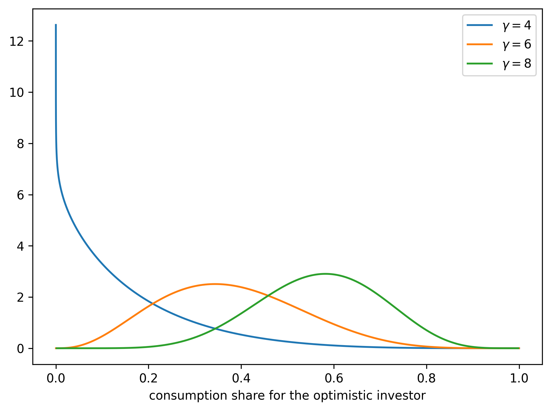
Fig. 8.1 Stationary density for the fraction of output allocated to the mistakenly optimistic investor for alternative specifications of risk aversion. The risk aversion parameter is assumed to be the same for both investors. [1]#
8.5. Factoring a multiplicative functional#
Following [Hansen and Scheinkman, 2009] and [Hansen, 2012], we factor a multiplicative functional into three multiplicative components having the primitive types Example 8.1, Example 8.2, Example 8.3.
As in definition Definition 8.1, let \(Y\) be an additive functional, and let \(M = \exp(Y)\). Apply a one-period operator \(\mathbb{M}\) defined by
to bounded Borel measurable functions \(f\) of the Markov state. We recycle notation: Chapter 2 uses \({\mathbb M}\) for the resolvent operator \((1-\lambda)\sum_{j=0}^\infty \lambda^j {\mathbb T}^j\) that it deploys to characterize irreducibility. That operator and this one are unrelated. By applying the Law of Iterated Expectations, a two-period operator iterates \(\mathbb{M}\) twice to obtain:
with corresponding definitions of \(j\)-period operators \(\mathbb{M}^j\). The family of operators is a special case of what is called a “semi-group.” The domain of the semigroup can typically be extended to a larger family of functions, but this extension depends on further properties of the multiplicative process used to construct it.
We next derive a revealing representation of this semigroup by factoring the multiplicative functional \(M\) in an interesting way. We achieve this by applying what is referred to in mathematics as Perron-Frobenius theory based on the following equation:
Eigenvalue-eigenfunction Problem: Solve
for an eigenvalue \(\exp(\tilde \eta)\) and a positive eigenfunction \({\tilde e}\).
Consistent with Perron-Frobenius theory, call the positive eigenvalue the principal eigenvalue, and the associated positive eigenvector the principal eigenfunction, of the operator \(\mathbb{M}\).
Use the principal eigenvalue and eigenvector, and define:
Note that we constructed \({\widetilde N}_{t+1}\) so as to have a conditional expectation equal to unity. Using \({\widetilde N}\) as a martingale increment process, build
Theorem 8.1
Let \(M\) be a multiplicative functional. Suppose that the principal eigenvalue-eigenfunction problem has a solution with principal eigenfunction \({\tilde e}(X)\). Then the multiplicative functional is the product of three components that are instances of the primitive functionals in examples Example 8.1, Example 8.2, and Example 8.3:
where \({\widetilde L}_t\) is a multiplicative martingale with \({\widetilde L}_0 = 1\).
The factorization of a multiplicative functional described in Theorem 8.1 is a counterpart to the Chapter 4 Proposition 4.1 decomposition of an additive functional. We used the Proposition 4.1 martingale to identify the permanent component of an additive functional in Chapter 4. In this chapter, we shall use the multiplicative martingale isolated by Theorem 8.1 to represent a change of probability measure, one that will help us understand long-term risk-return tradeoffs. While \({\widetilde L}\) is a multiplicative martingale, \(\log {\widetilde L}\) is a supermartingale. There is a weaker connection between the two representations, however. Write the additive decomposition as:
where \({\widehat L}\) is an additive martingale. As [Hansen, 2012] argues, if \({\widetilde L}\) is not degenerate (not equal to one), then \({\widehat L}\) is not degenerate (not equal to zero) and conversely.
Models in which \(X\) is a finite-state Markov chain give a direct computation in which the principal eigenvalue calculation reduces to finding an eigenvector of a matrix with all positive entries.
Example 8.5
The stochastic process \(X\) is governed by a finite-state Markov chain on state space \( \{ {\sf u}_1, {\sf u}_2, \ldots, {\sf u}_n \}\), where \({\sf u}_i\) is the \(n \times 1\) vector whose components are all zero except for \(1\) in the \(i^{th}\) row. The transition matrix is \({\mathbb P},\) where \({\sf p}_{ij} = \textrm{Prob}( X_{t+1} = {\sf u}_j | X_t = {\sf u}_i)\). We represent the Markov chain as
where \({\mathbb E} (X_{t+1} | X_t ) = {\mathbb P}' X_t \), \({\mathbb P}'\) denotes the transpose of \({\mathbb P}\), and \(W_{t+1}\) is an \(n \times 1\) vector process that satisfies \({\mathbb E} ( W_{t+1} | X_t) = 0 \), which is therefore a martingale-difference sequence adapted to \(X_t, X_{t-1}, \ldots , X_0\). Think of \(W_{t+1}\) as the vector of errors when forecasting \(X_{t+1}\) based on current information.
Let \({\mathbb G}\) be an \(n \times n\) matrix whose \((i,j)\) entry \({\sf g}_{ij}\) is an additive contribution to the growth that \(Y_{t+1} - Y_t\) experiences when \(X_{t+1} = {\sf u}_j\) and \(X_t = {\sf u}_i\). The stochastic process \(Y\) is governed by the additive functional
Let \(M= \exp(Y)\). Define a matrix \({\mathbb M}\) whose \((i,j)^{th}\) element is \({\sf m}_{ij} = \exp({\sf g}_{ij}).\) Represent the stochastic process \(M\) as the multiplicative functional:
Associated with this multiplicative functional is the principal eigenvalue problem
To convert this to a linear algebra problem, write the \(j^{th}\) entry of \({\tilde e}\) as \({\tilde e}_j\). Since \(X_t\) always assumes the value of one of the coordinate vectors \({\sf u}_i, i =1, \ldots, n\),
when \(X_t = {\sf u}_i\) and \(X_{t+1} = {\sf u}_j\). This allows us to rewrite the principal eigenvalue problem as
or
where \(\widetilde {\sf m}_{ij} \eqdef {\sf p}_{ij} {\sf m}_{ij}\) and \({\tilde e}_i\) is entry \(i\) of \({\tilde e}\).
Notice that this construction incorporates the transition probabilities into the construction of the matrix \({\widetilde {\mathbb M}}\). We do this to reduce the problem to one of finding an eigenvalue and corresponding eigenvector of a matrix. Specifically, we want the positive eigenvalue associated with a positive eigenvector of (8.11).
After solving the principal eigenvalue problem, we construct an alternative transition matrix for a finite-state Markov process. Construct
and form the matrix \({\widehat {\mathbb N}} = [{\widehat {\sf n}}_{ij}]\). The matrix \({\widehat {\mathbb N}}\) has entries that are nonnegative, and
which verifies that \({\widehat {\mathbb N}}\) can be viewed as a transition matrix.
Finally, we show how to construct the factorization of the \(M\) process. To build the martingale of interest, we must undo the probability scaling that we did when forming \({\widehat {\mathbb N}}.\) With this in mind, solve for \({\tilde n}_{ij}\) that satisfies:
where we arbitrarily set \({\widetilde {\sf n}}_{ij}\) equal to one when \({\sf p}_{ij} = 0\) and build the matrix \({\widetilde {\mathbb N}} = [ {\widetilde {\sf n}}_{ij}]\). These constructions allow us to write (8.10) as
Remark 8.3
In the previous example, suppose that \({M_{t+1}}/{M_t} \) is a one-period stochastic discount factor used to represent asset prices via a formula:
for alternative one-period asset payoffs \({G_{t+1}}/{G_t}\) that are constructed in terms of \(X_{t+1}\) and \(X_t\). In the previous construction, the matrix \(\widetilde {\mathbb M}\) could be inferred from prices of one-period-ahead Arrow securities. Specifically, given prices of all of the state contingent claims for next period, we can infer the row of \(\widetilde {\mathbb M}\) associated with a given current state. By looking across states, we can fill out all of the rows of \(\widetilde {\mathbb M}\). We only need to know \(\widetilde {\mathbb M}\) to pose and solve the principal eigenvalue problem and hence to construct transition probabilities as given by (8.12), but not the \({\sf p}_{ij}\)’s and the \({\sf m}_{ij}\)’s. This provides a challenge for recovering transition probabilities from asset prices. The \({\sf p}_{ij}\)’s and \({\sf m}_{ij}\)’s cannot be inferred uniquely from the \({\widetilde {\sf m}}_{ij}\)’s. In particular, the Arrow prices are insufficient to identify the transition probabilities. [Ross, 2015] imposed additional restrictions on \({\widetilde{\sf m}}_{ij}\)’s that implied that the recovered probabilities are actually the \({\sf p}_{ij}\)’s. In general, the recovered probabilities will differ from the baseline transition probability matrix because these restrictions fail to be satisfied. We will have more to say about this difference and investigate why the recovered probabilities remain interesting. See [Borovička et al., 2016] for an extended discussion of this claim.
The following log-linear, log-normal specification displays the mechanics of the multiplicative factorization and its connection to the corresponding additive decomposition.
8.5.1. An application#
Sargent et al. [2025] fit a model of this form to US Consumer Expenditure Survey data and then apply decomposition (8.15) to it. For each date \(t\) they sort households and form \(M\) quantiles of the cross sections of private income, post-tax income, and consumption. From the private-income quantiles they construct a Chisini mean \(Y_t\) that they interpret as aggregate income. They then subtract \(Y_t\) from every quantile of all three variables, subtract each quantile’s time-series mean, and stack what remains under the demeaned growth rate \(Y_t - Y_{t-1} - \nu\) to form a state vector \({\sf y}_t\) of dimension \(3M+1\). They assume that \({\sf y}_t\) is governed by a first-order vector autoregression
where \(e_1\) selects the first entry of the state.
With \(M = 100\) bins the state has \(301\) components, far more than the number of quarterly observations, so an unrestricted \({\sf B}\) is underdetermined. That is what leads them to impose reduced rank on \({\sf B}\) and to estimate it by a dynamic mode decomposition.[2]
Their transition matrix \({\sf B}\) is our \({\mathbb A}\), and their shocks \({\sf a}_{t+1}\) enter the state directly rather than through a loading matrix. Setting \({\mathbb A} = {\sf B}\), \({\mathbb D} = e_1{\sf B}\), \({\mathbb F} = e_1\), and \({\mathbb B} = {\mathbb I}\) in (8.15) reproduces their decomposition exactly, including the coefficient vectors
Fig. 8.2 plots the result. The left panel estimates \(\nu\), \({\sf B}\), and the shock covariance from data through 2008Q4 and then applies (8.15) to the full sample; the right panel estimates them from the whole 1990–2023 sample. Read the left panel first. Shortly before 2008 the martingale component sits near zero and \(Y_t\) runs above the pre-crisis trend \(t\nu\). After 2008 the martingale falls to about \(-15\) percent and never returns, while the stationary component declines gradually and turns negative at the end of 2014. By 2023 \(Y_t\) is roughly 20 percent below the trend line extrapolated from pre-crisis data. The two panels differ in what they attribute to \(\nu\): estimating on the full sample lowers the trend, so less of the post-2008 shortfall is left for the martingale to carry.
The figure makes visible what Proposition 4.1 of Chapter 4 asserts algebraically. A permanent shock is an innovation to the martingale, and the martingale is the only component of (8.15) that does not revert. Whether a decline in a measured aggregate is permanent or transitory is therefore a question about which component absorbed it, and the decomposition answers that question rather than leaving it to a judgment about how long “temporary” lasts.
The same coefficient \({\mathbb H}\) then governs welfare. Sargent et al. [2025] exponentiate to form the multiplicative functional \(C_t = \exp(c_{p,t})\) for a household at quantile \(p\), and compute the compensating difference in consumption that leaves a risk-sensitive consumer indifferent between the estimated process and one with a given source of risk removed. The recursive utility example of Chapter 4 shows why \({\mathbb H}\) is what matters: as the subjective discount factor approaches one, the risk adjustment (4.10) to a continuation value becomes \((1-\gamma)/2\) times \(\left|{\mathbb H}\right|^2\), the variance of the martingale increment (4.6). Compensations for bearing i.i.d. growth risk depend on the one-period shock variance, while compensations for bearing the serially correlated risk carried by \(\sum_{j \le t}{\mathbb H}{\sf a}_j\) depend on \({\mathbb H}\), which cumulates the shock’s effect over all horizons. The gap between the two is large, and it is the same gap that separates \(\left|\alpha(1)\right|^2\) from \(\sum_j\left|\alpha_j\right|^2\) in Proposition 3.2 of Chapter 3. Chapter 11 develops the risk-sensitive recursion that produces these compensations.
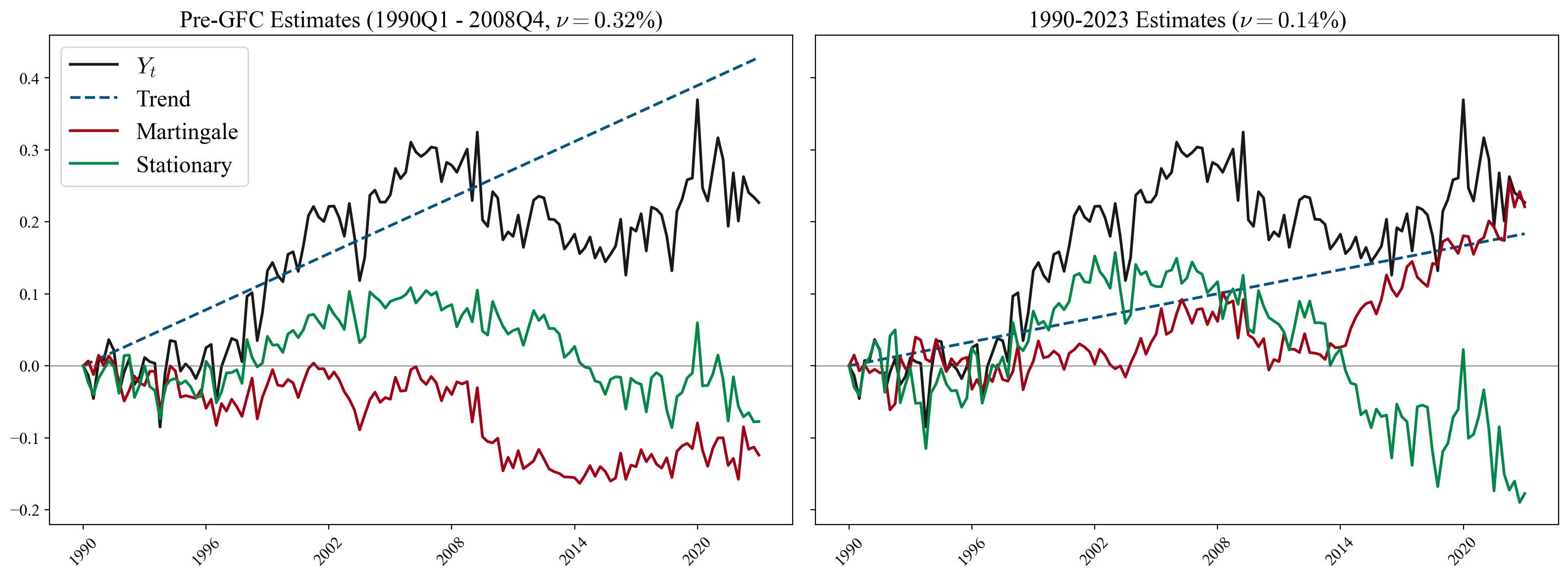
Fig. 8.2 Decomposition (8.15) of \(Y_t - Y_0\) into trend, martingale, and stationary components, for a model fit to US Consumer Expenditure Survey cross sections. Left panel: parameters estimated from 1990Q1–2008Q4, then applied to the full sample. Right panel: parameters estimated from 1990–2023. Computed using the replication package of Sargent et al. [2025].#
Let \(M_t = \exp(Y_t)\). Use equation (8.15) to deduce
where
and
The additive martingale of \(Y= \log(M)\) has a variance that grows linearly over time. That variance contributes a component to the exponential trend of the multiplicative functional \(M\), along with a simple time-horizon adjustment to the martingale component.
Example 8.6
Consider a stationary \(X\) process and an additive \(Y\) process described by the VAR
where \({\mathbb A}\) is a stable matrix and \(\{ W_{t+1} : t \ge 0 \}\) is a sequence of independent and identically distributed normal random vectors with mean zero and covariance matrix \({\mathbb I}\). In Proposition 4.1 of Chapter 4, we described the decomposition
where
Example 8.7
Consider the following stochastic volatility example. Suppose that a scalar state variable evolves as a first-order autoregression:
where \(\{W_{t+1} : t \ge 0 \}\) is an i.i.d. sequence of normally distributed random variables. The state variable \(X_t\) gives the source of volatility fluctuations. Guess a principal eigenfunction of the form:
and construct
Write the principal eigenfunction equation as:
where we took logarithms of both sides of the equation. The computation on left side of this equation has a tractable formula for expressing the outcome as a quadratic function of the state.
Solve the equation in three steps. First, equate coefficients on \(x^2\) and deduce a quadratic equation for \(\epsilon_2.\) Next, equate the coefficient on \(x\) and obtain a linear equation for \(\epsilon_1\). Finally, equating the constant terms to obtain an equation for \({\tilde \eta}\). The initial quadratic equation is
When it has a solution, there will typically be two possible choices. For the solution to be of interest, \(1 - \epsilon_2 {\sf b}^2\) must be positive.
Second, equate the coefficient on \(x\) to solve an equation for \(\epsilon_1\) given \(\epsilon_2\):
Third, we solve for \({\tilde \eta}\) by equating the constant and plugging the solutions for \(\epsilon_1\) and \(\epsilon_2\):
For this example,
where \(\propto\) means equal up to a scale factor that depends on \(X_t\). Under the implied change in measure, \(W_{t+1}\) is distributed as a normal random variable with conditional mean
and precision \(1 - \epsilon_2 {\sf b}^2\). Under the change of probability measure, \(W_{t+1}\) remains normally distributed, with a different variance and a state-dependent mean, and \(X\) remains a first-order autoregression with different dynamics. It could, for instance, be an explosive autoregression.
Remark 8.4
The martingale component of the multiplicative functional has “peculiar behavior.” It has expectation one by construction. The Martingale Convergence Theorem guarantees that sample paths converge, typically to zero. This theorem is operative because the positive martingale is bounded from below. Since its date zero conditional expectation is one, for long horizons this process necessarily has a fat right tail. Fig. 8.3 plots probability density functions of the martingale component for different values of \(t\).
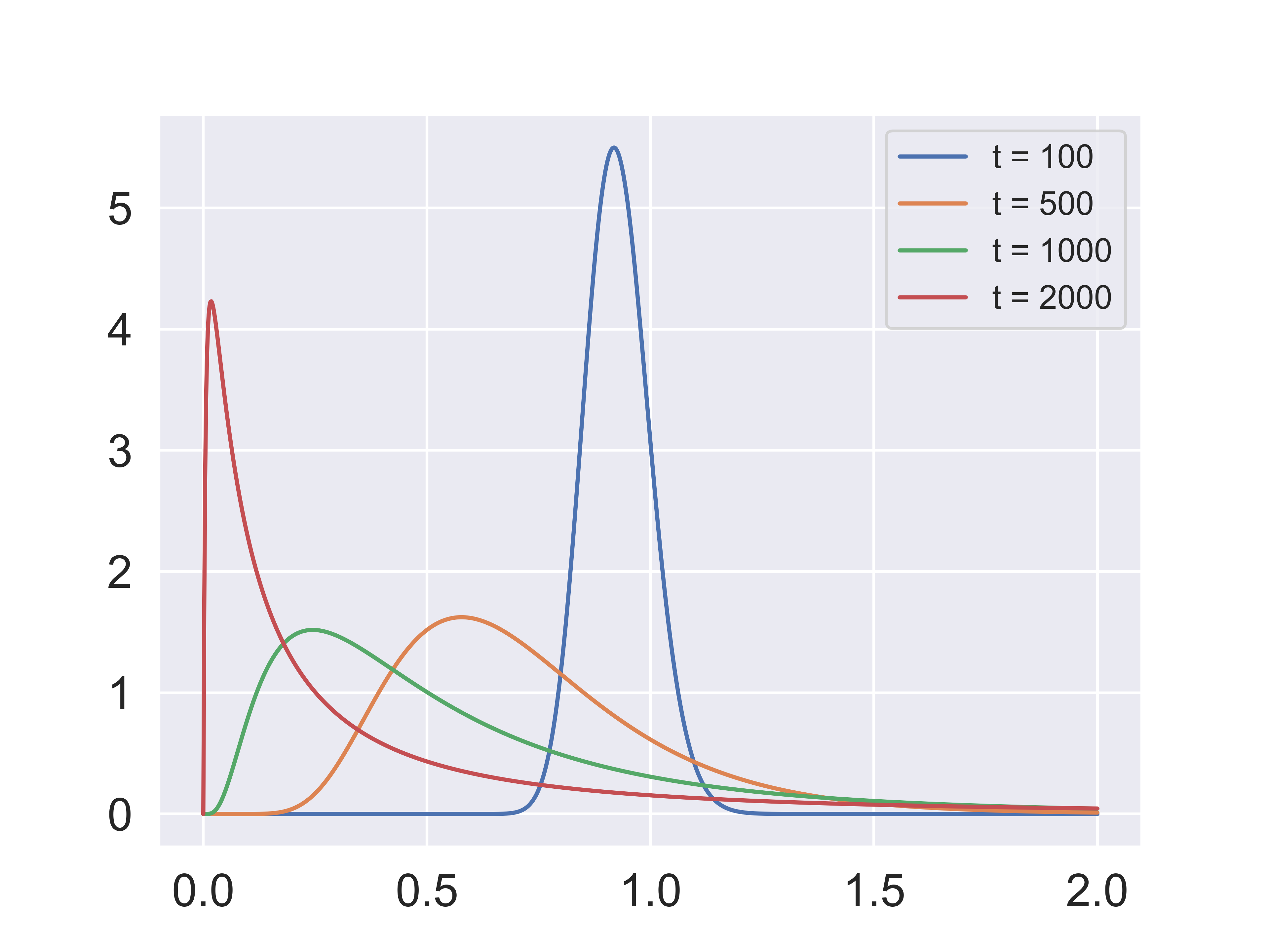
Fig. 8.3 Density of \(\widetilde{L}_t\) for different values of \(t\).#
Consider the behavior of cumulative returns over long horizons. Since \(SR\) is a positive martingale, as illustrated by Fig. 8.3, it becomes increasingly important that the process has excursions for which it becomes large as we extend the horizon. This is the setting for the [Martin, 2012] argument about fat tails in scaled cumulative returns that we noted in Chapter 7; Section Illustrating the decompositions: a worked example quantifies it.
While the multiplicative martingale has peculiar sample path properties, we are primarily interested in this martingale component as a change of probability measure. For instance, in Example 8.6, formula (8.14) for \({\widetilde N}_{t+1}\) tells how the change in probability measure induces mean \( {\mathbb H}\) in the conditional distribution for the shock \(W_{t+1}\). Similarly, \({\widetilde {\mathbb N}},\) with entries given in formula (8.12), provides an alternative transition matrix in Example 8.5.
8.6. Illustrating the decompositions: a worked example#
The additive decomposition of Chapter 4 and the multiplicative factorization Theorem 8.1 of this chapter become concrete and easy to visualize once we specialize Example 8.6 to a simple scalar process and simulate it. The example that follows is of the kind studied by [Hansen, 2012]; it displays the irregular but persistent growth typical of economic time series such as output, prices, and dividends, while remaining simple enough to decompose by hand.
8.6.1. A concrete additive functional#
Let the additive functional \(Y\) be driven by a scalar fourth-order autoregression written in companion form. With state \(X_t = \left( {\tilde X}_t, {\tilde X}_{t-1}, {\tilde X}_{t-2}, {\tilde X}_{t-3} \right)'\) and a scalar shock \(W_{t+1} \sim {\mathcal N}(0,1)\), set
so that \(X_{t+1} = {\mathbb A} X_t + {\mathbb B} W_{t+1}\) and \(Y_{t+1} - Y_t = \nu + {\mathbb D} X_t + {\mathbb F} W_{t+1}\), exactly the structure of Example 8.6. We take \(\nu = .01\) and \(\sigma = .01\); the autoregressive coefficients \((.5, -.2, 0, .5)\) have an associated polynomial with all roots outside the unit circle, so \({\mathbb A}\) is stable.
Applying the Chapter 4 decomposition Proposition 4.1, reproduced as (8.15), splits \(Y\) into four pieces,
with martingale loading \({\mathbb H} = {\mathbb F} + {\mathbb D}({\mathbb I} - {\mathbb A})^{-1}{\mathbb B}\) and stationary loading \(g(x) = {\mathbb D}({\mathbb I} - {\mathbb A})^{-1} x\). For our numbers, \({\mathbb H} = .05\) and \(g = \begin{bmatrix} 4 & 1.5 & 2.5 & 2.5\end{bmatrix}\). Fig. 8.4 plots a single simulated path of \(Y_t\) together with its trend, martingale, and stationary components. The linear trend \(\nu t\) supplies deterministic drift; the martingale \(\sum_{j=1}^t {\mathbb H} W_j\) accumulates the permanent effects of the shocks and wanders ever farther from its origin, its standard deviation growing like \(\sqrt t\); the stationary component \(-g(X_t)\) fluctuates within a fixed band and captures the transient dynamics.
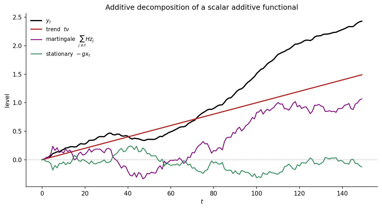
Fig. 8.4 The four-part additive decomposition (8.16) of a simulated path of the additive functional \(Y_t\): a deterministic trend \(\nu t\), a martingale \(\sum_{j=1}^t {\mathbb H} W_j\) with permanent effects, and an asymptotically stationary component \(-g(X_t)\). (The constant \(g(X_0)\) is zero here because \(X_0 = 0\).)#
8.6.2. The associated multiplicative functional#
Let \(M_t = \exp(Y_t)\). By Theorem 8.1, \(M\) factors as
with, exactly as in Example 8.6,
The exponential growth rate \({\tilde \eta} = \nu + |{\mathbb H}|^2 / 2 = .01125\) exceeds the additive trend rate \(\nu = .01\): the gap \(|{\mathbb H}|^2 / 2\) is the Jensen adjustment that converts the linearly growing variance of the additive martingale into an exponential contribution to the geometric growth of \(M\). The martingale increment \({\widetilde N}_{t+1} = \exp\left( {\mathbb H} W_{t+1} - |{\mathbb H}|^2/2 \right)\) is precisely the exponential martingale (8.14); viewed as a change of probability measure, it re-centers the innovation, shifting its conditional mean from \(0\) to \({\mathbb H}\).
8.6.3. The peculiar property and higher moments#
We now return to the “peculiar behavior” of the multiplicative martingale \({\widetilde L}\) noted in Remark 8.4: although \(E_0 {\widetilde L}_t = 1\) for every \(t\), its sample paths converge to zero almost surely. Fig. 8.5 displays many simulated paths of \({\widetilde L}_t\) over a long horizon. The theoretical mean, marked by the dash-dotted line, stays pinned at one, yet almost every path drifts toward zero; the unit mean is preserved only by an ever thinner set of paths that take ever larger values.
The Gaussian structure makes the mechanism transparent. Because
\({\widetilde L}_t\) is log normal. The mean \(-a_t/2\) of \(\log {\widetilde L}_t\) drifts downward at exactly the rate that keeps \(E_0 {\widetilde L}_t = \exp\left( - a_t/2 + a_t/2 \right) = 1\). Herein lies the peculiarity: the median value \(\exp(-a_t/2)\) collapses to zero while the mean stays at one.
The tension is resolved by the higher moments. For any integer \(k \ge 1\),
so the mean (\(k=1\)) equals one for all \(t\), while every higher moment grows exponentially in \(a_t = t\,|{\mathbb H}|^2\). The variance, skewness, and (raw) kurtosis are
Fig. 8.6 plots these on a natural logarithmic scale. Variance, skewness, and kurtosis all climb without bound as \(t\) grows, and they do so faster the larger \(|{\mathbb H}|^2\) is. Since (8.17) and these summary statistics depend on \({\mathbb H}\) only through \(|{\mathbb H}|^2\), the strength of the permanent component alone governs how quickly the distribution of \({\widetilde L}_t\) becomes right skewed. This is the picture anticipated by Fig. 8.3: as \(t\) increases, \({\widetilde L}_t\) becomes ever more right skewed, with most of its probability mass collapsing toward zero and a long, fattening right tail carrying just enough mass to hold the mean at one. It is why, as [Martin, 2012] emphasized, scaled cumulative returns on long-dated assets inherit fat right tails, and why a sample average of \({\widetilde L}_t\) computed from a finite collection of paths typically falls well short of the unit population mean.
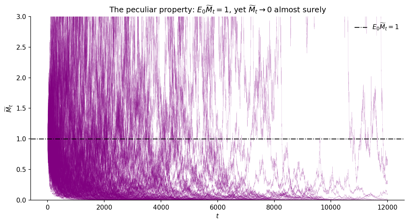
Fig. 8.5 The peculiar property of the multiplicative martingale \(\widetilde L_t\): its conditional mean is \(E_0\widetilde L_t = 1\) for all \(t\) (dash-dotted line), yet almost every path converges to zero as \(t\) grows. The permanent-component loading is held at the chapter’s calibration, \(|\mathbb{H}| = .05\), so that \(a_t = t|\mathbb{H}|^2\); drag paths to change how many trajectories are shown.#
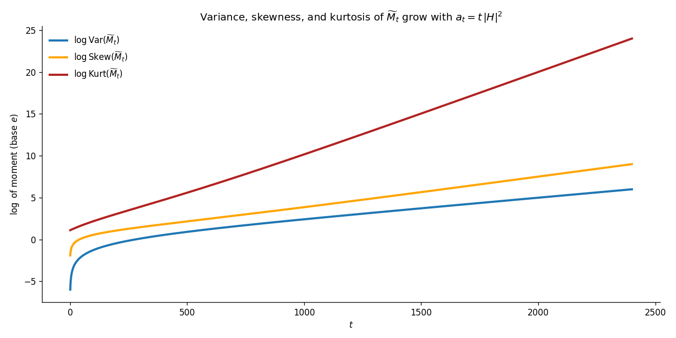
Fig. 8.6 Variance, skewness, and kurtosis of \({\widetilde L}_t\), on a natural log scale, all grow without bound with \(a_t = t \, |{\mathbb H}|^2\), even though \(E_0 {\widetilde L}_t = 1\) for every \(t\). The rapidly rising higher moments are the quantitative counterpart of the increasingly right-skewed densities that underlie the peculiar property.#
8.7. Stochastic stability#
Our characterization of a change of probability measure as the solution of a Perron-Frobenius problem determines only transition probabilities. Since the process is Markov, it is of interest to seek an initial distribution of \(X_0\) under which the process is stationary and satisfies a stochastic stability property that we will define and explore. Stochastic stability opens the door to the study of a variety of limiting behavior and hence justifies our interest in the multiplicative factorization. The eigenfunction problem can have multiple solutions; it turns out, however, that there is a unique solution for which the process \(X\) is stochastically stable under the implied change of measure. See [Hansen and Scheinkman, 2009] and [Hansen, 2012] for formal analyses of this problem in a continuous-time Markov setting. In what follows we investigate the discrete-time counterpart to their investigations.
Definition 8.2
A process \(X\) is stochastically stable under a probability measure \({\widetilde {Pr}}\) if it is stationary and \(\lim_{j \rightarrow \infty} {\widetilde {\mathbb E}} \left[f(X_j) \mid X_0 = x \right] = {\widetilde {\mathbb E}} \left[ f(X_0) \right]\) for any Borel measurable \(f\) satisfying \({\widetilde {\mathbb E}} \vert f(X_t) \vert < \infty\).
As we discussed previously, a multiplicative martingale \(L\) with \(L_0 =1\) induces a probability measure conditioned on \(X_0.\) To check for stochastic stability, we extend the probability by including a distribution over \(X_0\) in a manner that ensures the process \(X\) is stationary.
Remark 8.5
Notice that the stationary probability distribution for \(X_t\) implied by \(\widetilde {Pr}\) is used to define the limits of the conditional expectations. For the mathematical results, however, how we initialize the distribution over \(X_0\) is not crucial. Thus, we could equivalently consider other probability measures under which \(X_t\) has the same limiting distribution as \(t\) gets large. Under such probability measures, the process \(X\) would be asymptotically stationary. In this sense, we impose the stronger stationarity restriction as a matter of convenience.
Theorem 8.2
Let \(M\) be a multiplicative functional. Suppose that \((\tilde \eta, \tilde e)\) solves the eigenfunction problem and that under the change of measure \(\widetilde{Pr}\) implied by the associated martingale \(\widetilde L\) the stochastic process \(X\) is stationary and ergodic. Consider any other solution \((\eta^*, e^*)\) to eigenfunction problem with implied martingale \(\{ L_t^* \}\). Then
\(\eta^* \ge \tilde \eta\).
If \(X\) is stochastically stable under the change of measure \(Pr^*\) implied by the martingale \(L^*\), then \(\eta^* = \tilde \eta\), \(e^*\) is proportional to \(\tilde e\), and \(L^*_t = \widetilde L_t\) for all \(t=0,1,... \).
Proof. First we show that \(\eta^* \ge \tilde \eta\). Write:
Thus,
If \(\tilde \eta > \eta^*\), then
But this equality cannot be true because under \(\widetilde{Pr},\) \(X\) is stochastically stable and \(\frac {e^*}{\tilde e}\) is strictly positive. Therefore, \(\eta^* \ge {\tilde \eta}.\)
Consider next the case in which \(\eta^* > \tilde \eta\). Write
which implies that
Thus,
If \(\tilde \eta < \eta^*\), then
so that \(X\) cannot be stochastically stable under the \(Pr^*\) measure.
Finally, suppose that \(\tilde \eta = \eta^*\) and that \(\frac {\tilde e(x)}{e^*(x)}\) is not constant. Then
and \(X\) cannot be stochastically stable under the \(Pr^*\) measure.
Stochastic stability under the martingale-induced change of measure provides a way to frame some interesting long-term approximations. Let
where \({\widetilde L}\) is the martingale component in the factorization of \(M\). Construct the operator:
where we have used the factorization of \(M\) to construct an alternative conditional expectation operator. Form the family (semi group) of operators:
where we used the factorization given by Theorem 8.1 and the unique selection of such a representation Theorem 8.2 to obtain the right-side equality. Since \(X\) is stochastically stable under \(\widetilde{Pr}\),
for all \( \tilde e f\) provided that \(f \in {\mathcal F} ({\widetilde L} ).\) We use limit (8.19) to justify calling the Perron-Frobenius eigenvalue the long-term growth or decay rate of the multiplicative functional.
Under the stochastic stability restriction, we obtain a more refined approximation by adjusting for the growth or decay in the family of operators:
where we assume that \(f\) is in \({\mathcal F}({\widetilde L})\). Thus once we adjust for the impact of \({\tilde \eta}\), the limiting function is proportional to \({\tilde e}\). The function \(f\) determines only a scale factor \({\widetilde {\mathbb E}}\left[f(X_t) \right]\).
We will apply the limiting results in a variety of ways in this and subsequent chapters. The multiplicative factorization can help us understand implications of stochastic equilibrium models for valuations of random payout processes. In addition, such factorizations can help organize empirical evidence in ways that make contact with such stochastic equilibrium asset pricing models. We also use these tools to calculate Chernoff entropy as introduced in Chapter 7. Worked computations of these entropies appear in the Appendix to Chapter 11.
8.8. Inferences about permanent shocks from asset prices#
Macroeconomists often study dynamic impacts of shocks to systems of variables measured in logarithms. For example, [Alvarez and Jermann, 2005] suggest looking at asset prices using a multiplicative representation of a cumulative stochastic discount factor, though without the tools provided by this chapter. The additive decomposition derived and analyzed in Chapter 4 is a convenient tool for identifying permanent shocks. A prominent multiplicative martingale component implies a prominent role for permanent shocks in the underlying economic dynamics. A formal probability model lets us link an additive decomposition as described in this chapter and Chapter 4 to the multiplicative factorization that we study in this chapter. Log normal models, at least as approximations, are often used by applied macroeconomists. Example 8.6 provides an example with explicit formulas linking the two representations. While distinct, the two martingales, in this special case, are closely linked. In general, the connection is more subtle. In what follows we describe how a multiplicative martingale component to a stochastic discount factor is reflected in asset prices.
Consider the following stochastic discount factorization
where \(S_0= L_0^s = 1.\) A date zero price of a long-term bond is:
Compute the corresponding yield by taking \(1/t\) times minus the logarithm:
Provided that
the limiting yield on a discount bond is \(- \eta^s.\)
Next consider a one-period holding period return on a \(t\) period discount bond:
Using stochastic stability and taking limits as \(t\) tends to \(\infty\) gives the limiting holding-period return:
A simple calculation shows that \(R_1^{\infty}\) satisfies the following equilibrium pricing restriction on a one-period return:
These long-horizon limits provide approximations to the eigenvalue for the stochastic discount factor and the ratio of the eigenfunctions.
In a model without a martingale component, [Kazemi, 1992] observed that the inverse of this holding-period return is the one-period stochastic discount factor; that is, within the [Kazemi, 1992] setup, \((R_1^\infty)^{-1}\) equals the one-period stochastic discount factor. Let \(Y_1\) be a vector of asset payoffs and \(Q_0\) be the corresponding vector of prices. Then standard asset pricing theory implies the conditional moment restrictions
[Alvarez and Jermann, 2005] extend this insight by showing that the reciprocal reveals the component of the one-period stochastic discount factor net of its martingale component.
Remark 8.6
In practice, we only have bond data with a finite payoff horizon, whereas the characterizations [Kazemi, 1992] and [Alvarez and Jermann, 2005] use bond prices with a limiting payoff horizon. Empirical implementations using such characterizations assume that the observed term structure data have a sufficiently long duration component to provide a plausible proxy for the limiting counterpart.
8.9. Chernoff entropy reconsidered#
In Chapter 7, we introduced Chernoff entropy as a statistical measure of distance between two probabilities. We now return to that discussion by extracting an asymptotic decay rate from a multiplicative factorization. Let \(L\) be a martingale constructed as a likelihood ratio process and construct:
The martingale \(L\) represents the probabilities of an alternative model relative to a baseline one. Its increment is
Let \({\tilde \eta}(\alpha)\) be the principal eigenvalue exponent in the Theorem 8.1 factorization of \(M = L^\alpha\), selected as in Theorem 8.2, so that \({\tilde \eta}(\alpha) \le 0\). Consistent with the convention of Chapter 7, the asymptotic decay rate is the nonnegative quantity
and the corresponding Chernoff entropy is given by
It gives the asymptotic rate of discrimination between the baseline model and the alternative as more data become available. Large decay rates say that learning eventually becomes easy; small rates say that it does not.
Example 8.8
A researcher considers two possible autoregressive models of a scalar time series:
Let \(f_1(y \mid x)\) and \(f_2(y \mid x)\) be conditional normal densities given by:
where \(\phi\) denotes the standard normal density. Define the kernel
We seek the principal eigenfunction \(g\) and eigenvalue \(\lambda\) satisfying
It may be verified that the principal eigenfunction is an exponential quadratic function of the state. The eigenvalue problem may be solved uniquely by restricting the eigenvalue to be positive. The constructed martingale in the factorization induces an alternative stable autoregression. The following figure illustrates the computation and the resulting Chernoff entropies for alternative values of the AR coefficient. The reported \({\sf a}_{\alpha^*}\)’s give the corresponding AR coefficients for the stability verifications.
Example 8.9
A researcher considers two possible autoregressive models of a scalar time series:
where the autoregression coefficient is known and the same for each model, but the value of \({\sf b}\) is not. We entertain two possible values for \({\sf b}\). We proceed analogously to the previous example. In this case, the principal eigenfunction is constant with a unique solution for the eigenvalue. The following figure illustrates the computation and the resulting Chernoff entropies for alternative values of the conditional volatility parameter \({\sf b}\). The reported \({\sf b}_{\alpha^*}\)’s give the corresponding uncertainty exposure coefficients for the stability verifications. The entropies are notably higher than for the unknown AR coefficient case in the previous example, suggesting that the time series data are more informative for the conditional volatility coefficient.
8.10. Digression on rational expectations#
Under a rational expectations assumption, a researcher equates the baseline probability measure with the one implied by the equilibrium of the model. The model of [Kazemi, 1992] provides an example. Kazemi’s underlying baseline model is Markov. Kazemi assumes that economic agents living inside his model are completely confident that they know those Markov dynamics. He thus adopts a rational expectations assumption. As noted by [Lucas, 1987] (p. 13)
The term ‘rational expectations’, as Muth used it, refers to a consistency axiom for economic models, so it can be given precise meaning only in the context of specific models. I think this is why attempts to define rational expectations in a model-free way tend to come out either vacuous (‘People do the best they can with the information they have’) or silly (‘People know the true structure of the world they live in’).
Once we add the assumption that our model-implied expectations actually generate the data we are studying, the rational expectations formulation of Muth and Lucas opens the door to a comprehensive econometric approach. Consider an econometrician who does not know some or all of the parameters of the underlying economic model and who proceeds to infer those parameters using formal statistical methods that have come to be called rational expectations econometrics. To elaborate, we call probabilities that are model-consistent in the sense of Muth and Lucas “model-implied probabilities”. These probabilities can in principle be expressed as a function of the model’s parameters. The outcome is typically a set of cross-equation restrictions that link formally the beliefs of the economic agents within the model to the data generation. Computing these restrictions involves solving a set of nonlinear equations that include Euler equations like the asset pricing equation (8.21) above as well as other equations that help determine the complete Markov dynamics. Being able to compute these functions is what opens the door to the application of formal statistical methods such as maximum likelihood. Importantly, this approach assumes that at least one of the members of the parameterized set of statistical models is consistent with the data generating process and that it is this data generation that the economic agents within the model use in their decision making. An application of rational expectations econometrics thus relies heavily on the economist’s model being complete in the sense of [Geweke, 2010]. [Sargent, 1978], [Saracoglu and Sargent, 1978], [Sargent, 1979], [Hansen and Sargent, 1980], [Wallis, 1980], [Hansen and Sargent, 2019] and other contributions in [Lucas and Sargent, 1981] present early applications of this complete-specification approach. [Hansen and Sargent, 2013], ch. 9 describes time-domain and frequency domain maximum likelihood estimation for a class of linear-quadratic-Gaussian dynamic stochastic general equilibrium models. These procedures are widely used throughout applied macro and monetary economics, due in part to the convenient software provided by [Adjemian et al., 2024] and [Herbst and Schorfheide, 2016].
[Hansen and Singleton, 1982] and [Hansen and Richard, 1987] suggest a different approach. They assume that an econometrician only has partial information and does not impose or fully parameterize the baseline probability model. Implicitly, they allow for the model components that are not fully parameterized to be revealed imperfectly (except in the infinite sample limit) to the econometrician by the actual data generating process. Thus, [Hansen and Singleton, 1982] and [Hansen and Richard, 1987] replace Muth’s consistency axiom operational in a fully specified econometric model with another notion of consistency that is implied by a Law of Large Numbers limit in a statistical setting that assumes that the process described by the baseline model is stationary and ergodic. Formally, this approach is implemented with a vector of conditional moment restrictions. [Hansen and Singleton, 1982] and [Hansen and Richard, 1987] thereby make possible a limited-information alternative to imposing rational expectations with a fully specified baseline model. Such an approach continues to adopt the simplification that economic agents, in contrast to an econometrician, know the underlying data generating process. Relieved of having to specify the full economic dynamic system, this limited information approach gains further flexibility by applying the law of iterated expectations to derive implications that the econometrician can use for estimation and testing. Applying such an approach in the context of the [Kazemi, 1992] setup converts the degenerate martingale restriction imposed by Kazemi into a moment restriction that accommodates estimation and statistical testing by using the generalized method of moments. See [Hansen, 1982].
Many published papers in the applied macro, industrial organization, and asset pricing literatures apply one of these two approaches. “Rational expectations econometrics” assumes that the econometrician knows a parameterized family of models that includes the rational expectations equilibrium, and that only the agents know the correct member of that family. The alternative approach assumes that the econometrician has only a partial a priori specification and leverages the Law of Large Numbers to fill in the rest.
The rational expectations econometrics assumptions that a correctly-specified model is among the parameterized family and that the economic agents inside the model know key parameters that the econometrician does not are heroic, to put it politely. Even Lucas’s statement above expresses skepticism when he dismisses the statement that ‘People know the true structure of the world they live in’ as being silly. Sophisticated applied economists acknowledge up front that their models are approximations, meaning that they are misspecified. Instead of formally integrating their concerns about possible misspecifications into statistical implementations, for reasons of tractability users of rational expectations econometrics routinely ignore such approximation concerns. For skeptics, the rational expectations econometrics straitjacket is simply too confining, leading them to adopt less formal methods of model matching and validation. Relatedly, without ever claiming or providing evidence that their model-implied expectations agree with an actual data generation process, many papers in applied theory routinely impose rational expectations in the process of constructing models of so-called stylized facts.
As we argued previously, a subjective belief specification is often expressible as a multiplicative martingale relative to a baseline probability specification, say the rational expectations counterpart or the probability that captures the actual data generation. Thus subjective beliefs offer one candidate for a multiplicative martingale component to the cumulative stochastic discount factor within the [Kazemi, 1992] setup. Statistical divergences provide a way to measure the magnitude of the belief-induced misspecification needed to capture empirical failures that arise from using one of the rational expectations econometrics approaches just described. This opens the door to using a statistical perspective to assess the role of subjective probabilities in models without rational expectations, in contrast to much of the existing research on subjective beliefs in asset pricing. See Bounding investor beliefs for an elaboration. To its credit, rational expectations provides a framework for conducting counterfactuals using an underlying dynamic economic model, along the lines of [Marschak, 1953] and [Hurwicz, 1966]. More general subjective belief formulations including ones represented by multiplicative martingales, unfortunately, struggle to do something comparable. Deciding when to use misspecified models and for what purposes is an important challenge for applied researchers.
8.11. Values of stochastic cash flows#
In a fundamental paper, [Rubinstein, 1976] featured the importance of cash-flow pricing in contrast to the often studied return-based analyses.
8.11.1. Long-term risk-return tradeoff for cash flows#
Following [Hansen and Scheinkman, 2009] and [Hansen et al., 2008], we consider the valuation of stochastic cash flows, \(G\), that are multiplicative functionals. Such cash flows are determinants of prices of both equities and bonds.
We now study valuation from the perspective of the long-term limits measured by the logarithms of the eigenvalues, the \(\tilde \eta\)’s, the long-term limits of prices of such cash flows. Consider a cash-flow growth process \(G\) measured as a multiplicative functional. The corresponding cash-flow return over horizon \(t\) is:
where we have normalized \(S_0 = 1\). Note that as a special case, the cash-flow return on a unit date \(t\) cash-flow is:
Define the proportional risk premium on the initial cash-flow return as the expected return divided by the riskless counterpart for the same horizon. Taking logarithms and adjusting for the time horizon gives:
where in the first expression, the first term is the logarithm of the expected payoff, the second term is minus the logarithm of the price, and the third term is minus the logarithm of the riskless cash-flow return for horizon \(t\). Scaling by \(1/t\) adjusts for the investment horizon.
The product \(SG\) is itself a multiplicative functional. Let \(\eta^{sg}\) denote its geometric growth component. Then from (8.22), the limiting cash-flow risk compensation is:
This holds under the moment restrictions imposed in limit (8.19). The expression resembles the negative of a covariance as is often found in asset pricing, but it differs from a covariance because we are working with proportional measures of the risk compensations. When the cash flow process, \(G,\) is a cumulative return, the asset pricing restrictions inform us that \(SG\) is a martingale. In this case, the proportional risk premium is just:
where, as we noted previously, \(- \eta^s\) is the long-term counterpart to a riskless rate of return.
8.11.2. Finite versus infinite-valued claims#
In a recent paper, [Panageas, 2025] reminds us that several important issues bear on finite values of claims to infinite cash flows, including macro processes like aggregate consumption and aggregate output. These issues include speculative bubbles, dynamic efficiency, and equity claims linked to macroeconomic outcomes. Importantly, he argues that the adjustment for uncertainty can play an important and sometimes subtle role in such evaluations.[3] We now explore in more detail when such valuations are finite taking account of uncertainty adjustments.
We start by building stochastic counterparts to the well known and pedagogically revealing Gordon growth model posed in discrete time. By using the framework developed in this chapter, we characterize the uncertainty adjustments necessary for such valuations. In so doing, we show how the tools of Black-Scholes option pricing must be altered to understand these valuations.
We build a multiplicative functional using the product, \(M = G S,\) where \(G\) captures stochastic growth in the cash flow and \(S\) stochastic discounting. The factorization in Theorem 8.1 and the selection we featured in Theorem 8.2 provide a defense for using \(\tilde \eta\) as an asymptotic growth or decay rate of \(M\) provided that we select the solution that is stochastically stable. To justify finite values of equity-based assets for a family of cash flows, we restrict \(\tilde \eta<0\) so that stochastic discounting dominates stochastic growth. We now revisit that analysis, deconstruct the outcome, and explore the limitations.
8.11.2.1. Constant discounting#
As a warm-up, consider a discrete-time Gordon growth model where:
with \(\eta_s <0\) reflecting discounting and \(\eta_g\) capturing growth. The well known and simple to compute outcome gives:
for \(M = SG\), provided that \({\tilde \eta} = { \eta}_s + {\eta}_g < 0\). Thus we have the familiar restriction that discounting has to dominate growth in a deterministic setting.
As is also well-known, the separation is not quite so simple because growth contributes to the rate of return used for discounting. The term \(\eta_s\) could reflect both subjective discounting in preferences and an adjustment contributed by economic growth in consumption that can either enhance or diminish the discount rate depending on investor preferences for intertemporal substitution.
8.11.2.2. Expected discounted cash flows#
Next consider discounted expected values for \(\tilde \eta < 0 \) and a stochastically stable Markov process \(X\). Recall that stochastic stability implies that conditional expectations converge to their unconditional counterpart. Thus we, temporarily, abstract from uncertainty adjustments in valuation not reflected in conditional expectations or encoded in the discount rate (We will be agnostic about how we come up with \(\tilde \eta\)). Consider the valuation of a positive claim on the Markov state, say \(f(X)\)
Under the presumed stochastic stability of the Markov process, two possibilities are of interest:
While it is common to feature the finite-moment case, here we proceed more generally. Except for the finite-state Markov case, we may easily construct payoffs that are positive functions of the Markov state that have infinite expectations. When the unconditional expectation is infinite, the value of the equity-type claim may or may not be finite. The expectation’s rate of divergence races the discount rate \(- {\tilde \eta}\). When the former grows faster than \(- {\tilde \eta},\) the valuation in (8.23) will be infinite, even though the underlying Markov process is stochastically stable.
Our more general approach required that we address a multiplicity that emerges when we factor \(M\). Take \(M_t =
\exp\left( \tilde \eta t \right) \phi(X_t).\) For the sake of discussion, take \(S_t = \exp\left( \tilde \eta t\right)\), and \(G_t = \phi(X_t)\).
As a special case for such an \(M\) process, consider the solutions to the following equation:
Setting \({\hat e} = 1\) and \({\hat \eta} = 0\) solves this equation, but there can be other solutions. For solutions with \( \hat \eta > 0\), the conditional expectations diverge geometrically and they must have infinite unconditional moments. More generally, the potential divergence of the conditional moments is precisely the source of multiple factorizations for \(M,\) and what drives our choice of selecting one. The associated cash flow with a date \(t\) contribution, \(\phi(X_t) = {\hat e}(X_t),\) will have infinite value when \(\hat \eta > - {\tilde \eta}\).
Example 8.10
Consider a special case of Example 8.7 with \(\nu = {\sf f}_0 = {\sf f}_1 = 0. \) This makes \(M=1\). We look for solutions of the form:
The quadratic equation of interest simplifies to:
This has two solutions. One is \(\epsilon_2 = 0.\) For this one, \({\hat \eta}=0\) and \({\hat e} = 1\) and gives rise to the solution that we expect. For the other one,
\(\epsilon_1 = 0\), and
because \({\sf a}^2 < 1\).
8.11.2.3. A simple stochastic extension of the Gordon growth model#
To model stochastic growth and discounting, consider the very special case of two correlated geometric random walks with constant expected discounting or growth rates. Suppose
where \(\mu_s\) and \(\mu_g\) are constants with \(\mu_s < 0,\) \(\mu_g > 0\), and \(\sigma_s\) and \(\sigma_g\) are constant row vectors and the \(W\) process is iid with \(W_{t+1}\) being a standard multivariate normally distributed random vector. Form the product process, \(M = SG,\) which will have the same mathematical structure:
Construct
The first term in the second line captures the negative of the implied risk-free rate of return, the second term the expected growth rate, and the third term, \(\sigma_s \cdot \sigma_g,\) includes an adjustment for uncertainty. The security with cash flow \(G\) has finite value when \(\tilde \eta < 0\) with the familiar geometric summation formula:
This computation illustrates a way to build a stochastic version of the Gordon growth model, but it has important limitations from both a conceptual and empirical perspective.
8.11.2.4. Adjusting for uncertainty with state dependence#
The stochastic example in the previous subsection has pedagogical value, but the interest rates are constant as are the cash-flow growth rates. The same is true for the one-period cash-flow exposures to the shock vector \(W_{t+1}\). We escape this straitjacket by introducing state dependence expressed as follows:
By using the factorization of Theorem 8.1 and the unique Theorem 8.2 selection of such a representation, we return to our initial present-value analysis in Expected discounted cash flows. Write
where \(M = SG\). Consider a family of cash flows of the form
for different choices of \( f = {\tilde f } {\tilde e} \) and \(\tilde f \in {\mathcal F}(\widetilde L)\) given by (8.18). Stated in terms of logarithms, the cash flows are all cointegrated, with cointegrating coefficients one and minus one. The process \(G\) reflects a common stochastic growth component. [Hansen, 2012] explores in detail relations between cointegration as it is studied in macroeconomics and long-term valuation as it is of interest in this chapter. In particular, the set \({\mathcal F}(\widetilde L)\) imposes moment restrictions for the valuation limits. Distinct moment implications arise in other applications of cointegration.
The uncertainty-adjusted valuation of the discounted cash flows of the form given in (8.25) is given by:
where the expectation uses the probability distribution induced by \({\widetilde L}\). Infinite values arise whenever \({\tilde \eta} \ge 0\). When \({\tilde \eta} < 0\) the valuation is finite provided that \({\widetilde {\mathbb E}} [ {\tilde f}(X_t) ]\) is finite. Thus, \({\tilde \eta}\) as a measure of the asymptotic growth or decay in \(SG,\) plays a central role in determining whether the discounted expected value of the cash-flow \(G\) is finite or not. But like the analysis in Expected discounted cash flows, there is a nuanced case in which
For this infinite-moment case, whether the discounted expected value is finite or not depends on the rate of divergence in comparison to \(- {\tilde \eta}\).
Importantly, this analysis uses a change in probability measure for the computation. The change of measure mathematically resembles a standard risk-neutral probability, but it is conceptually distinct. It depends on the stochastic behavior of \(SG\) and not just \(S\). Moreover, state-dependent short-term interest rates alone imply that the risk-neutral probabilities are not the relevant ones for valuing long-term cash flows. With state-dependence in stochastic growth, it becomes valuable to move from \(S\) to \(SG,\) which builds on the Gordon-growth insight. The uncertainty adjustments for valuation depend on the implied asymptotic rate of growth or decay, \(-{\tilde \eta},\) analogous to what happens in deterministic environments. It could, however, also depend on the corresponding behavior of the conditional expectations,
of the cash flows as the payoff horizon becomes large.
Although stated in the context of a very special example, the analysis in [Panageas, 2025] reminds us that in a stochastic setting, unconditional moments can be infinite even when there is stochastic stability in the Markov process and the horizon-dependent conditional moments are finite. This means the value comparison for stochastic cash-flows with different specifications of \(f\) could be dramatically different because of the tail behavior of the stationary distributions of random variables \(f(X_t)/{\tilde e}(X_t)\) for the different \(f\)’s. More than the rate \({\tilde \eta}\) may come into play. It would appear to be hard to tell how restrictive the finite moment condition is empirically, but that does not mean we should dismiss it as a possibility. It sometimes matters when we build explicit models of valuation as illustrated by [Panageas, 2025].
8.11.3. Partitioning long-term return implications#
We study a family of cash-flow and holding period returns where the cash flows are of the form (8.25) under some moment restrictions on \(f(X_t)\). Specifically, we show that limiting returns are the same as the payoff horizon becomes long, for alternative choices of \(f > 0.\) [Jiang et al., 2024] use the valuation impact of cointegration in the relation between government spending and revenue to assess the implied value of government debt in comparison to actual direct measurements.
8.11.3.1. Cash-flow returns#
Consider two factorizations:
Given \(G\), entertain a family of cash flows that can be represented as in (8.25) for \(f>0\)-s such that
The two factorizations of interest for cash flows (8.25) are:
Implicit in these factorizations is that the introduction of \(f\) has neither impact on the Perron-Frobenius eigenvalues nor any effect on the multiplicative martingales. It does change the eigenfunction by replacing \(e^g\) with \(e^g/f\). With these extensions along with moment restrictions (8.26), the limiting expected growth and valuation rates are:
Observe that the limits remain the same for alternative choices of \(f>0\) as does the expected rate of return given by:
8.11.3.2. One-period holding-period returns#
We also investigate the limiting behavior of one-period holding-period returns and obtain an even stronger connection among the family of returns for cash flows satisfying (8.25). To achieve this, we revisit and extend a computation we performed previously. Consider the multiplicative factorization again and price future cash flows in single periods. (These are sometimes referred to as “strips.”) An empirical asset pricing literature has explored these returns starting with [van Binsbergen et al., 2012]. See [Golez and Jackwerth, 2024] for a recent update of this evidence.
The one-period holding period return on a \(t\)-period asset with payout \(G_tf(X_t)\) at date \(t\) is:
where the \(\tilde \cdot\) conditional expectation uses the probability measure induced by the positive martingale \(L^{sg}\). Using stochastic stability and taking limits as \(t\) tends to \(\infty\) gives the limiting holding-period return:
provided that \(f/e^{sg} \in {\mathcal F}(L^{sg})\). The limiting holding-period return does not depend on \(f\).
Much of this chapter has featured factorizations that allow us to deconstruct economically interesting processes including growth processes. We now consider a way to parametrize cash-flow growth processes in terms of holding-period returns and decay rates. We do this to reveal common long-term risk exposures in positive cash-flow growth processes. Formally, we build partitions of such processes. For a given cumulative stochastic discount factor process \(S\) with \(S_0=1,\) parameterize baseline stochastic cash flows as
where
\(\eta\) is a positive decay rate;
\(R\) is a one-period return process constructed as
for some \(\kappa\);
the implied multiplicative martingale with increment
and \(L_0 = 1\) induces a stochastically stable process for \(X\).
Notice that for a given cumulative stochastic discount factor process \(S,\) the martingale \(L\) reveals the cumulative return process \(R\) and conversely. Since we restrict \(R\) via its implications for the martingale \(L\), we use the notation \(G(\eta,L)\) to denote the baseline process. The initial condition \(G_0(\eta, L) > 0\) is inconsequential at this juncture.
For each baseline process, introduce a family of cash-flow growth processes within a partition:
Notice that for each \(G\) in a partition \({\mathcal G}(\eta, L),\) we have the factorization:
for some \(f \in {\mathcal F}(L).\) Each such member has the same one-period holding period return, \(R\).
A given cash-flow process \(G\) reveals the corresponding \((\eta, L)\) and the partition to which \(G\) belongs. Consider two cash flow processes \(G^1\) and \(G^2\) within the universe of all of the partitions that are related by:
Thus they are cointegrated in logarithms with vector \((1, -1)\). These processes are necessarily within the same partition with a common \((\eta, L)\).
Remark 8.7
[Ai and Fu, 2025] extend the holding-return limits derived here to study what can be revealed by announcement impacts on financial markets. They use a continuous-time formulation with hidden states and preset announcement dates at which information is revealed about monetary policy. They study instantaneous returns at the times of the announcements. They deduce counterpart representations applicable to such holding-period returns. They use this setup to estimate long-term impacts of monetary policy announcements on the macro economy as revealed by such returns. Their analysis is facilitated by their use of log-linear models with Brownian motion increments, which opens the door to a tractable link between the multiplicative martingale increments and permanent shocks revealed by additive decompositions applied to logarithms.
8.12. Bounding investor beliefs#
We use the cumulative stochastic discount factorization to analyze two distance approaches to drawing inferences about investor beliefs.
8.12.1. Subjective beliefs in the absence of long-term risk#
Suppose that we have data on prices of one-period state-contingent claims. We can use these data to infer the one-period operator, \({\mathbb M}.\) Recall that we represent this operator using a baseline specification of the one-period transition probabilities. One possibility is that the one-period baseline transition probabilities agree with the data generation. Rational expectations models equate transition probabilities to those used by investors. More generally, investors could have subjective beliefs that differ from the baseline specification. We proceed under two restrictions:
investors think there are no permanent macroeconomic shocks;
investors do not have risk-based preferences that can induce a multiplicative martingale in a cumulative stochastic discount factor process.[4]
Under these two restrictions, we could identify \(L^s\) as the likelihood ratio for investor beliefs relative to the baseline probability distribution. Thus, the implied martingale component in the cumulative stochastic discount factor identifies the subjective beliefs of investors. Using this change of measure, the limiting long-term risk compensations derived in the previous section are zero. These assumptions facilitate “Ross recovery” of investor beliefs.[5]
8.12.2. Restricting the martingale increment with limited asset market data#
Initially, suppose we impose rational expectations by endowing investors with knowledge of the data generating process. With limited asset market data, we cannot identify the martingale component of the cumulative stochastic discount factor process without additional model restrictions. We can, however, obtain potentially useful bounds on the martingale increment. For applications beyond those of [Alvarez and Jermann, 2005], [Bakshi and Chabi-Yo, 2012], see [Koijen et al., 2010] and [Lustig et al., 2019], among others. We know that the implied martingale has some peculiar limiting behavior and that martingale and transient components can be correlated. Nevertheless, the implied probability measure can be well behaved. Consequently, in contrast to the references just cited, we use the increment as a device to represent conditional probabilities instead of just as a random variable. Extensions of these same methods can be used to study restrictions on subjective beliefs implied by asset prices.
There is a substantial literature on divergence measures for probability densities. Relative entropy is an important example. More generally, consider a convex function \(\phi\) that is zero when evaluated at one. Jensen’s inequality implies that
and equal to zero when \(N_1\) is one, provided that \(N_1\) is a multiplicative martingale increment (has conditional expectation one). This gives rise to a family of \(\phi\) divergences that can be used to assess departures from baseline probabilities. Relative entropy, \(\phi(n) = n \log n\), is an example that is particularly tractable and has been used often. Both \(n \log n\) and \(- \log n\) can be interpreted as expected log-likelihood ratios. The same family of divergences reappears in Chapter 10, where it restrains a decision maker’s search over priors and over likelihoods, and again in Chapter 13, where it measures the misspecification of a set of moment conditions.
One way of assessing the magnitude of the martingale increment to the stochastic discount factor is to solve:
Minimum divergence problem
subject to:
where \(Y_1\) is a vector of asset payoffs and \(Q_0\) is a vector of corresponding prices, and where \({\widehat S_1}/{\widehat S_0}\) is equal to one of the two possibilities:
i) \(\exp(\eta^s) \frac{ e^s(X_0)} {e^s(X_1)}\) under the data generating process;
or
ii) an imposed stochastic discount factor allowing for subjective beliefs to differ from the data generating process.
With regards to i), recall that the term
can be approximated by the reciprocal of the one-period holding-period return on a long-term bond. With regards to ii), for a model that is misspecified under the data generating process, we can ask that the distortion induced by the subjective beliefs correct the misspecification under the data generating process.
Remark 8.8
It is enlightening to extend problem (8.28) to include an inequality constraint requiring that the conditional expectation of any random variable of interest be less than or equal to some threshold. Adding a constraint, when it binds, increases the objective. A given increase in the divergence is achieved by reducing this threshold sufficiently far. By following this procedure, we can find a lower bound on the moment of interest that increases the objective by some pre-specified percentage. Extending this approach to any bounded random variable reveals an ambiguity-induced nonlinear expectation operator, where the nonlinearity follows from our construction of a lower bound on conditional expectations. Obtaining an ambiguity interval for a given random variable follows from also constructing the lower bound for the negative of this random variable. See [Chen et al., 2020] for a more extensive discussion. Such constructions are an example of what econometricians describe as partial identification because the vector \(Y_1\) of asset payoffs used in the analysis may not be sufficient to reconstruct all potential one-period asset payoffs and prices. In effect, the econometrician is often confronted with incomplete data on financial markets.
Remark 8.9
Many researchers use \(\phi(n) = - \log n\) as a divergence measure. [Chauduri et al., 2023] and [Chen et al., 2024], however, isolate a problem with monotone decreasing divergences such as \(- \log n\): they can fail to detect certain limiting forms of deviations from baseline probabilities.
Remark 8.10
[Ghosh and Roussellet, 2023] suggest a formal econometric procedure for estimating the altered probability measure obtained by minimum divergence. Presumably their methods could be extended to produce conditional ambiguity intervals as well.
Remark 8.11
To avoid having to estimate conditional expectations, applications often study unconditional expectations. In such situations, conditioning can be brought in through the “back door” by scaling payoffs and prices with variables in the conditioning information set; for example, see [Hansen and Singleton, 1982] and [Hansen and Richard, 1987]. See [Bakshi and Chabi-Yo, 2012] and [Bakshi et al., 2017] for some related implementations.
Remark 8.12
[Alvarez and Jermann, 2005] use \(- {\mathbb E}\left( \log S_1 - \log S_0 \right) \) as the objective to be minimized. Notice that
where the term in square brackets is the logarithm of the limiting holding-period bond return (8.20). The criterion thus equals that in the minimum divergence problem, but with an additive translation. Rewrite the constraints in the minimum divergence problem as:
This leaves us with an equivalent minimization problem in which the translation term is subtracted off to obtain the bound of interest.
Applied researchers have sometimes omitted the first constraint, which weakens the bound.
8.12.2.1. Intertemporal divergence measures#
[Chen et al., 2020] propose extensions of the one-period divergence measures to multi-period counterparts that remain tractable and enlightening. By looking over time, the dynamic formulation essentially averages over the conditioning information; but it allows for subjectivity in the transition probabilities. Their dynamic measure of divergence is constructed as follows. For a given \(N\) process, let
This construction provides the implied transition probability adjustments for the alternative time horizons. To represent the one-period divergence in an alternative but equivalent way, construct a function \(\psi\) such that
The function \(\psi\) plays a role analogous to \(\phi\) when the roles between the \(N\)-implied probability and the baseline probability are interchanged. It may be shown that \(\psi\) is also strictly convex. Note also that \(\psi(1) = \phi(1) = 0\). By design,
With these building blocks, [Chen et al., 2020] suggest the divergence measure:
An alternative equivalent representation may be obtained by taking a Law of Large Numbers limit under the altered probability measure. When \(\phi(n) = n \log n,\) this divergence measure coincides with the one that is pertinent for the study of Donsker-Varadhan formulations of large deviations in Markov environments. This dynamic formulation of divergences opens the door to recursions for the bounds in the divergence minimization described in Remark 8.8.
8.12.2.2. Subjective belief bounds on proportional risk premia#
The next two figures report proportional risk compensations for the market return using an illustration from [Chen et al., 2020] under a presumed data generation and when distorted investor beliefs are permitted and risk aversion is constrained to be one. The compensations condition on dividend/price ratios. The figures include upper and lower endpoints of conditional expectations computed by extending the divergence minimization problem along the lines suggested by Remark 8.8 given by the upper and lower edges of shaded rectangles. The horizontal lines within the shaded rectangles give the conditional moments implied by the minimum divergence change in probability measure. By comparing the two figures, we see how ambiguity intervals decrease when we weaken the constraint on the divergence. Since the divergence measure used in the computation is explicitly dynamic, the associated subjective probabilities for the transition probabilities are also substantially altered. The implied stationary probabilities for the three states are
Notice that the altered probabilities reflect a substantial reduction in the probability of being in the high dividend-price state, making the big conditional divergence for the high dividend-price state seem to have a smaller effect on the dynamic divergence measure.
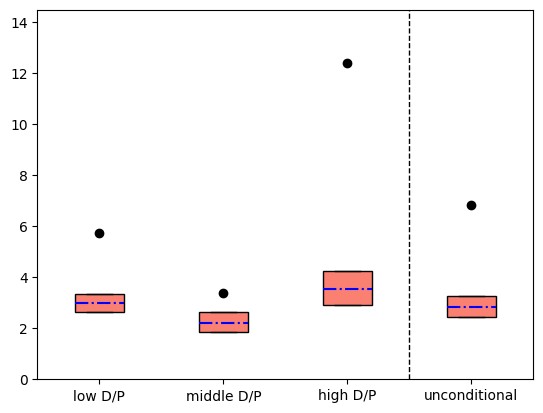
Fig. 8.7 Proportional risk compensations computed as \(\log \mathbb{E} R^m - \log \mathbb{E} R^f\) scaled to annualized percentages. The \(\bullet\)s are the empirical averages and the boxes give the imputed bounds when we inflated the minimum relative entropy by 20%.#
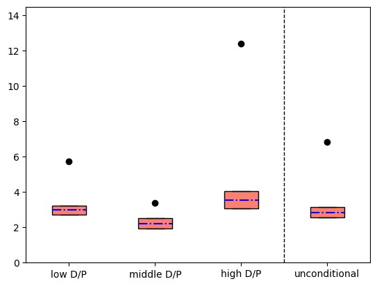
Fig. 8.8 Proportional risk compensations computed as \(\log \mathbb{E} R^m - \log \mathbb{E} R^f\) scaled to annualized percentages. The \(\bullet\)s are the empirical averages and the boxes give the imputed bounds when we inflated the minimum relative entropy by 10%.#
8.12.2.3. Subjective belief factor#
[Cui et al., 2025] use a complementary approach to study subjective beliefs and asset prices. They use a convenient mathematical representation of linear functionals. Consistent with our previous discussion, distorted expectations are viewed as a (conditional) linear mapping from the random variables being forecast to associated conditional predictions. A belief factor is identified as the random variable that appears in this representation of a conditional linear functional in a mathematical formulation in [Hansen and Richard, 1987] and [Cerreia-Vioglio et al., 2016]. [Cui et al., 2025] use this belief factor to organize useful descriptions of various data sets containing reports of subjective beliefs. In this setting, the subjective belief factor is restricted to be a (conditional) linear combination of the variables being forecast in the data set of interest, a restriction central to econometric identification. As [Cui et al., 2025] point out, extending the subjective belief functional to include forecasts of other variables omitted from a data set under study generates subjective belief factors whose best linear (conditional) predictors equal the subjective belief factor that they construct from their smaller data set. While identification remains partial in this setting, their framework provides convenient characterizations of what can be learned and why it is informative.
[Cui et al., 2025] correctly remind us that they do not restrict the subjective belief factor to be positive. They go on to suggest a way to impose positivity under some particular distributional assumptions. By using statistical divergences, the [Chen et al., 2020] analysis avoids these auxiliary assumptions while imposing positivity. It also provides an entirely different characterization of partial identification than does the approach of [Cui et al., 2025]. There are advantages and disadvantages to both approaches.
8.13. Measuring belief distortions with survey forecasts#
Bounding investor beliefs used asset prices to bound the multiplicative-martingale component of a cumulative stochastic discount factor. [Bhandari et al., 2025] add more structure to the problem to achieve full identification of a belief-distortion martingale, using household survey forecasts of macroeconomic variables.
Their evidence and the model that they use to interpret it fit squarely within the framework of this chapter: a decision maker’s subjective beliefs are represented by a multiplicative martingale \(L\) of the type introduced earlier in this chapter (see Example 8.2), and the discrepancy between subjective and objective forecasts is a conditional expectation of the martingale increment \(N_{t+1}\) against the variable being forecast. Because the martingale is now pinned down by survey data rather than inferred from prices, the exercise turns the abstract change of measure of this chapter into a directly measured object.
8.13.1. Belief wedges as covariances with the martingale increment#
Let \({\mathbb E} \left( \cdot \mid {\mathfrak A}_t \right)\) denote a conditional expectation under a baseline (data-generating or rational-expectations) probability, and let \({\widetilde {\mathbb E}} \left( \cdot \mid {\mathfrak A}_t\right) = {\mathbb E} \left(N_{t+1} \, \cdot \mid {\mathfrak A}_t \right)\) denote the corresponding subjective conditional expectation induced, as in formula (8.3), by a multiplicative-martingale increment \(N_{t+1} \ge 0\) with \({\mathbb E} \left(N_{t+1} \mid {\mathfrak A}_t \right) = 1\). Following [Bhandari et al., 2025], define the one-period belief wedge for a variable \(Z_{t+1}\) as the gap between the subjective and the baseline forecast:
Because \({\mathbb E} \left(N_{t+1} \mid {\mathfrak A}_t \right) = 1\), the wedge is exactly a conditional covariance between the martingale increment and the forecasted variable:
A positive wedge signals that the decision maker overweights states in which \(Z_{t+1}\) is high relative to the baseline probability. The martingale increment \(N_{t+1}\) studied throughout this chapter is more than a device for changing measures. Its covariation with observable variables is what a forecast survey measures.
8.13.2. The optimal distortion is an exponential multiplicative martingale#
[Bhandari et al., 2025] obtain a specific \(N_{t+1}\) from robust or multiplier preferences of the type initiated by [Hansen and Sargent, 2001] and developed in [Hansen and Sargent, 2008]. A decision maker who distrusts a baseline model replaces the ordinary continuation value \({\mathbb E} \left( {\widehat V}_{t+1} \mid {\mathfrak A}_t \right)\) by the outcome of the minimization
where \({\widehat V}_{t+1}\) is a continuation value and \(\theta_t > 0\) is a pessimism parameter that penalizes departures of \(N_{t+1}\) from unity as measured by conditional relative entropy. This is precisely the entropy-penalized problem (11.5) of Chapter 11, with \(\theta_t\) equal to the inverse penalty \(\frac 1 \xi = \gamma - 1\). Its minimizer is the exponentially tilted increment
which is nonnegative and has conditional expectation one, so it is a multiplicative-martingale increment of exactly the type of Example 8.2. Since (8.32) shifts probability toward states in which the continuation value \({\widehat V}_{t+1}\) is low, \(\theta_t > 0\) encodes pessimism. Allowing \(\theta_t\) to depend on the state, and in particular to change sign, lets the same construction express optimism (\(\theta_t < 0\)), which tilts probability toward high-continuation-value states. [Bhandari et al., 2025] reinterpret the robust-control distortion as a model of belief and let survey data discipline the process for \(\theta_t\); this also resolves an identification problem, because with unitary intertemporal elasticity these preferences are observationally equivalent to recursive utility with time-varying risk aversion \(\gamma_t = \theta_t + 1\), and survey forecasts, unlike prices, distinguish time-varying pessimism from time-varying risk premia.
Compounding the increments as in (8.4) builds the likelihood ratio process \(L_t = \prod_{j=1}^t N_j^*\), and formula (8.5) delivers the multi-period subjective forecasts
that the survey elicits at horizons beyond one period. The \(\tau\)-period wedge \(\Delta_t^{(\tau)}(Z) = {\widetilde {\mathbb E}}(Z_{t+\tau}\mid {\mathfrak A}_t) - {\mathbb E}(Z_{t+\tau} \mid {\mathfrak A}_t)\) is thus a compounded version of the one-period object (8.29), exactly as multi-period changes of measure compound one-period increments elsewhere in this chapter.
8.13.3. Gaussian dynamics: the distortion is a mean shift#
Suppose that the state follows the log-linear Gaussian law of motion
and that the continuation value is affine, \({\widehat V}_{t+1} \approx v_x X_{t+1} + \textrm{constant}\), with \(v_x\) a row vector of continuation-value sensitivities. Then the exponent in (8.32) is affine in \(W_{t+1}\), and the optimal increment collapses to
This is an exponential martingale of exactly the form (8.14) in Example 8.6: under the implied change of probability measure, the shock is simply re-centered,
so pessimism is a mean shift of the innovation equal to the negative of the pessimism parameter times the exposure \(v_x \psi_w\) of the continuation value to the shock. Fig. 8.9 illustrates the shift for the scalar calibration of [Bhandari et al., 2025].
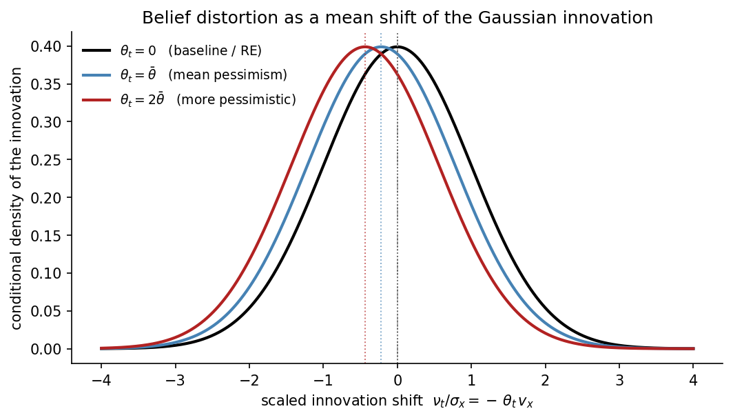
Fig. 8.9 The belief distortion (8.33) as a change of probability measure that shifts the mean of the Gaussian innovation. Larger pessimism \(\theta_t\) moves the perceived distribution of the shock to the left, toward states with lower continuation values. Because the true shift \(\nu_t = -\theta_t \left( v_x \psi_w \right)'\) is tiny at this calibration, the horizontal axis is scaled by \(1/\psi_w\), so the plotted shift is \(-\theta_t v_x\).#
The wedge (8.30) then has the closed form. For any variable \(Z_{t+1} = {\bar z}' X_{t+1}\) that is linear in the state,
so the belief wedge is the pessimism parameter times the conditional covariance between the forecasted variable and the continuation value. When \(Z_{t+1}\) is a “good” variable such as consumption (\(v_x > 0\)), the wedge is negative and the decision maker underforecasts it; when \(Z_{t+1}\) enters the continuation value with a negative sign, as unemployment does, the same pessimism produces a positive wedge, an overforecast. When the pessimism parameter is itself state dependent, \(\theta_t = {\bar \theta} X_t\), the mean shift (8.33) alters not just the intercept but also the persistence of the perceived law of motion, replacing \(\psi_x\) by \({\widetilde \psi}_x = \psi_x - \psi_w ( v_x \psi_w )' {\bar \theta}\); adverse states are more persistent under the subjective measure than under the baseline, so pessimists believe that bad times last longer.
8.13.4. One factor, and what survey data discipline#
Formula (8.34) has a sharp implication. The time variation in every belief wedge is governed by the single scalar \(\theta_t\), while the cross-sectional loadings \(-{\bar z}' \psi_w \psi_w' v_x'\) are conditional covariances between shocks and continuation values. These loadings are not free parameters: they are equilibrium objects determined by the model’s structure, so each additional surveyed variable adds an overidentifying restriction. A single common belief factor should therefore account for the joint movement of the wedges across variables.
[Bhandari et al., 2025] confirm this prediction in the Michigan Survey of Consumers. Household forecasts of unemployment and inflation display wedges that are positive on average, countercyclical (larger in recessions, when \(\theta_t\) is high), and dominated by a single principal component that accounts for roughly four-fifths of their joint variation. Calibrating the belief factor \(\theta_t\) to these moments and feeding it through a New Keynesian model, they find that the resulting belief shock substantially reduces the unemployment volatility puzzle of [Shimer, 2005] that standard technology and monetary-policy shocks cannot resolve.
This survey-based strategy is complementary to the asset-price bounds of Bounding investor beliefs. There, incomplete asset-market data delivered only a bound on the martingale increment of a stochastic discount factor; here, direct forecast data identify the belief martingale itself. In both cases the magnitude of the admissible distortion is governed by the same conditional relative entropy \({\mathbb E} \left(N_{t+1} \log N_{t+1} \mid {\mathfrak A}_t \right)\) that appears in the penalty (8.31), and the statistical detectability of the implied belief distortion is measured by the Chernoff entropy discussed earlier in this chapter. Persistent belief wedges of the size seen in surveys correspond to changes of measure that a statistician would find difficult to reject in samples of the length available, which is precisely why the distortions can survive as durable features of investor behavior.
Remark 8.13
The construction here is the same multiplicative martingale that Remark 8.2 used to study whether investors with distorted beliefs survive. Where [Borovička, 2020] characterizes preferences under which optimists are not driven out of the market in the long run, [Bhandari et al., 2025] use survey forecasts to measure the belief distortion period by period. Both exploit the fact, central to this chapter, that a subjective model is encoded in a multiplicative-martingale change of measure relative to a baseline probability.
8.14. Summary#
Exponentiating an additive functional gives a multiplicative functional, which grows or decays geometrically rather than linearly. Theorem 8.1 factors it into three pieces: a deterministic geometric trend \(\exp(t{\tilde \eta})\), a multiplicative martingale, and a ratio of a principal eigenfunction evaluated at the initial and current states. That eigenfunction solves (8.8), the growing counterpart of the unit-eigenvalue problem of Chapter 2, and Theorem 8.2 supplies the stochastic stability that makes the factorization the one to use for long-horizon questions.
The factorization does the work in each application. The martingale component determines long-term valuation and the limiting risk-return tradeoff; it also carries the belief distortions measured against survey forecasts. Chernoff entropy from Chapter 7 returns as a bound on how far distorted beliefs can stray before a statistician could detect them, which is why distortions of the size seen in surveys can persist. Chapter 9 perturbs these functionals to obtain shock elasticities.
8.15. Exercises#
Exercise 8.1 (Verifying the log-normal factorization)
Example 8.6 reports the factorization of \(M = \exp(Y)\) for the log-normal vector autoregression
with \({\mathbb A}\) stable, but does not verify it. Do so.
Write \({\sf g} \eqdef {\mathbb D}\left({\mathbb I}-{\mathbb A}\right)^{-1}\) and \({\mathbb H} \eqdef {\mathbb F} + {\sf g}{\mathbb B}\).
(a) Show that \({\mathbb D} + {\sf g}{\mathbb A} = {\sf g}\). Parts (b) and (c) use only this identity.
(b) Take \({\tilde e}(x) = \exp\left({\sf g}x\right)\) as a candidate principal eigenfunction and verify the eigenvalue equation (8.8) directly, computing \({\tilde \eta}\) along the way.
(c) Construct \({\widetilde N}_{t+1}\) from its definition and show that it reduces to the exponential martingale (8.14). Confirm that its conditional expectation is one.
(d) Compare \({\tilde \eta}\) with the trend coefficient \(\nu\) of the additive decomposition (8.15). Explain in words where the gap comes from, and why \({\mathbb H}\) and not \({\mathbb F}\) determines it.
Exercise 8.2 (A principal eigenvalue problem you can solve by hand)
Example 8.5 reduces the principal eigenvalue problem for a finite-state chain to the matrix problem (8.11). Work through a two-state case.
Let the chain have transition matrix \({\mathbb P}\) and let \({\mathbb G}\) collect the additive growth contributions \({\sf g}_{ij}\), so that \({\widetilde {\sf m}}_{ij} = {\sf p}_{ij}\exp\left({\sf g}_{ij}\right)\).
(a) Explain why \({\widetilde {\mathbb M}}\) has a strictly positive eigenvalue with a strictly positive eigenvector whenever \({\mathbb P}\) has all positive entries, and why that eigenvalue is the one wanted.
(b) Construct \({\widehat {\mathbb N}}\) from (8.12) and verify that its rows sum to one, so that it is a transition matrix. Where is the eigenvector equation used?
(c) Recover \({\widetilde {\mathbb N}}\) and assemble the factorization (8.13). Verify it entry by entry.
(d) Remark 8.3 observes that Arrow prices reveal \({\widetilde {\mathbb M}}\) but not \({\mathbb P}\) and \(\exp({\mathbb G})\) separately. Using your construction, exhibit two distinct pairs \(\left({\mathbb P}, {\mathbb G}\right)\) giving the same \({\widetilde {\mathbb M}}\), and say which objects in the factorization are nonetheless identified.
Exercise 8.3 (The peculiar property, quantified)
Section Illustrating the decompositions: a worked example states that \({\widetilde L}_t\) has unit mean for every \(t\) while almost every sample path converges to zero, and reports the moment formula (8.17). Establish these claims.
Let \(\log {\widetilde L}_t = \sum_{j=1}^t\left({\mathbb H}W_j - {\frac 1 2}\left|{\mathbb H}\right|^2\right)\) and write \({\sf a}_t \eqdef t\left|{\mathbb H}\right|^2\).
(a) Show that \(\log {\widetilde L}_t \sim {\mathcal N}\left(-{\sf a}_t/2, \, {\sf a}_t\right)\) and derive (8.17): \({\mathbb E}_0\left[{\widetilde L}_t^k\right] = \exp\left({\frac 1 2}k(k-1){\sf a}_t\right)\) for integer \(k \ge 1\).
(b) Compute the median of \({\widetilde L}_t\) and its variance. Reconcile a median converging to zero with a mean fixed at one.
(c) Use Proposition 7.3 of Chapter 7 to confirm almost-sure convergence to zero, and identify the drift in \(\log {\widetilde L}_t\) that drives it.
(d) A researcher estimates \({\mathbb E}_0\left[{\widetilde L}_t\right]\) by averaging \({\widetilde L}_t\) across a finite ensemble of simulated paths and finds a number well below one, with the shortfall growing in \(t\). Explain why, and say what this implies for Monte Carlo evaluation of long-horizon expectations under a change of measure.
Exercise 8.4 (A second eigenfunction and infinite values)
Example 8.10 exhibits a second solution to the eigenvalue equation for a stable scalar autoregression. This exercise derives it and draws out its consequences for valuation.
Specialize Example 8.7 by setting \(\nu = {\sf f}_0 = {\sf f}_1 = 0\), so that \(M \equiv 1\) and the eigenvalue problem is
with \(|{\sf a}| < 1\) and \({\sf b} \ne 0\). Look for \({\hat e}(x) = \exp\left(\epsilon_1 x + {\frac{\epsilon_2} 2}x^2\right)\).
(a) Show that \(\epsilon_2\) solves \({\sf b}^2\epsilon_2^2 + \left({\sf a}^2-1\right)\epsilon_2 = 0\) and exhibit both roots. Which gives the solution one expects?
(b) For the nonzero root, show that \(\epsilon_1 = 0\), that \(1 - \epsilon_2{\sf b}^2 = {\sf a}^2 > 0\) so the required positivity holds, and that \({\hat \eta} = -{\frac 1 2}\log\left({\sf a}^2\right) > 0\).
(c) Compute the dynamics of \(X\) under the change of measure induced by this second solution. Show that the autoregressive coefficient becomes \(1/{\sf a}\). Which hypothesis of Theorem 8.2 fails, and how does that proposition adjudicate between the two roots?
(d) Section Expected discounted cash flows asks when the discounted value (8.23) of a positive claim \(f(X_t)\) is finite. Take \(f = {\hat e}\) from (b). Show that \({\mathbb E}\left[{\hat e}(X_t)\right] = +\infty\), and give the condition on the discount rate \({\tilde \eta}\) under which the discounted value is nonetheless finite. Comment on the warning in the chapter that stochastic stability of \(X\) is not by itself enough to guarantee finite values.
8.16. Answers#
Solution to Exercise 8.1 (Verifying the log-normal factorization)
(a) Factor out \({\mathbb D}\) and use the definition of \({\sf g}\):
(b) With \({\tilde e}(x) = \exp({\sf g}x)\),
By (a) the coefficient on \(x\) is \({\sf g}\), and by definition the coefficient on \(W_{t+1}\) is \({\mathbb H}\). Taking expectations with the log-normal formula,
which is (8.8) with
The eigenfunction is strictly positive, as Perron-Frobenius theory requires.
(c) By definition,
\({\mathbb D}+{\sf g}{\mathbb A}-{\sf g} = 0\) by (a), so \(X_t\) drops out and
which is (8.14). Its conditional expectation is \(\exp\left(\left|{\mathbb H}\right|^2/2 - \left|{\mathbb H}\right|^2/2\right) = 1\).
(d) The additive decomposition of \(Y = \log M\) has trend \(\nu\); the multiplicative factorization of \(M\) has exponential growth rate \({\tilde \eta} = \nu + \left|{\mathbb H}\right|^2/2\). The gap is a Jensen adjustment. The additive martingale \(\sum_{j\le t}{\mathbb H}W_j\) has variance growing linearly at rate \(\left|{\mathbb H}\right|^2\), and exponentiating a random variable whose variance grows linearly contributes an exponential trend at half that rate. So a component that is pure noise in logarithms becomes a component of growth in levels.
It is \({\mathbb H}\) and not \({\mathbb F}\) that appears because what compounds over long horizons is the martingale increment, which aggregates the entire impulse response \({\mathbb F} + {\mathbb D}\left({\mathbb I}-{\mathbb A}\right)^{-1}{\mathbb B}\), not the one-period shock loading \({\mathbb F}\). As the chapter puts it, the linearly growing variance of the additive martingale contributes to the exponential trend of the multiplicative functional. This is why processes with the same one-period volatility but different persistence grow at different geometric rates in levels.
Solution to Exercise 8.2 (A principal eigenvalue problem you can solve by hand)
(a) \({\widetilde {\sf m}}_{ij} = {\sf p}_{ij}\exp\left({\sf g}_{ij}\right)\) is strictly positive whenever \({\sf p}_{ij}\) is, since the exponential is. The Perron-Frobenius theorem for strictly positive matrices then supplies a real eigenvalue equal to the spectral radius, simple, with a strictly positive eigenvector unique up to scale, and no other eigenvalue of equal modulus. Positivity of the eigenvector is what makes it admissible as an eigenfunction in the sense of the eigenvalue problem, and simplicity is what makes the resulting factorization unique.
(b) Define \({\widehat {\sf n}}_{ij} = \exp\left(-{\tilde \eta}\right){\widetilde {\sf m}}_{ij}{\tilde e}_j/{\tilde e}_i\). Each entry is nonnegative. Summing across \(j\),
where the middle step is the eigenvector equation (8.11). The eigenvector equation states that the tilted and rescaled matrix has unit row sums. This is the discrete counterpart of the general fact that \({\widetilde N}\) was constructed to have conditional expectation one.
(c) Solve \({\widehat {\sf n}}_{ij} = {\widetilde {\sf n}}_{ij}{\sf p}_{ij}\) for \({\widetilde {\sf n}}_{ij}\), setting it to one where \({\sf p}_{ij}=0\). Then for \(X_t = {\sf u}_i\) and \(X_{t+1} = {\sf u}_j\),
which is (8.13) entry by entry.
(d) Only the product \({\sf p}_{ij}\exp\left({\sf g}_{ij}\right)\) enters \({\widetilde {\mathbb M}}\). So for any strictly positive matrix \({\mathbb K}\) whose rows sum to one, the pair
reproduces \({\widetilde {\mathbb M}}\) exactly while assigning entirely different transition probabilities and growth rates. Concretely, one can take \({\mathbb P}'\) to be any transition matrix at all and absorb the difference into \({\mathbb G}'\).
Everything computed from \({\widetilde {\mathbb M}}\) is identified by asset prices: the principal eigenvalue \({\tilde \eta}\), the eigenvector \({\tilde e}\) up to scale, and hence the transition matrix \({\widehat {\mathbb N}}\). What is not identified is the split of \({\widehat {\mathbb N}}\) into the objective probabilities \({\sf p}_{ij}\) and the martingale increments \({\widetilde {\sf n}}_{ij}\). [Ross, 2015] closes the gap by imposing restrictions that force \({\widetilde {\sf n}}_{ij} \equiv 1\); as Remark 8.3 notes, when those restrictions fail the recovered probabilities are \({\widehat {\mathbb N}}\) rather than \({\mathbb P}\), and Section Bounding investor beliefs takes up what the recovered object means in that case.
Solution to Exercise 8.3 (The peculiar property, quantified)
(a) Each increment \({\mathbb H}W_j - {\frac 1 2}\left|{\mathbb H}\right|^2\) is normal with mean \(-{\frac 1 2}\left|{\mathbb H}\right|^2\) and variance \(\left|{\mathbb H}\right|^2\), and the increments are independent. Summing \(t\) of them gives \({\mathcal N}\left(-{\sf a}_t/2, {\sf a}_t\right)\). For a normal \(Z \sim {\mathcal N}(\mu,\sigma^2)\) we have \({\mathbb E}\left[e^{kZ}\right] = \exp\left(k\mu + k^2\sigma^2/2\right)\), so
which is (8.17). At \(k = 1\) the exponent vanishes and the mean is one for every \(t\), as a martingale requires.
(b) The median of a log-normal is the exponential of the median of its logarithm, namely \(\exp\left(-{\sf a}_t/2\right)\), which converges to zero geometrically. The variance is \({\mathbb E}\left[{\widetilde L}_t^2\right] - 1 = e^{{\sf a}_t}-1\), which diverges.
The distribution becomes increasingly right skewed. Most of the probability mass slides toward zero while an ever thinner set of paths takes ever larger values. The product of a vanishing probability with a diverging value holds the mean at one. Fig. 8.3 plots this.
(c) By the Law of Large Numbers applied to the additive functional \(\log {\widetilde L}_t\),
almost surely. A negative asymptotic slope for the logarithm forces \({\widetilde L}_t \rightarrow 0\) almost surely, which is Proposition 7.3. The drift responsible is the Jensen correction \(-{\frac 1 2}\left|{\mathbb H}\right|^2\), the very term inserted to make the level a martingale. Making the level have constant mean requires giving the logarithm a downward drift, and it is the logarithm that governs almost-sure behavior.
(d) The sample mean of \(S\) independent draws of \({\widetilde L}_t\) is dominated by rare large realizations. With variance \(e^{{\sf a}_t}-1\), the relative standard error of the sample mean is \(\sqrt{\left(e^{{\sf a}_t}-1\right)/S}\), which grows exponentially in \(t\). Unless \(S\) grows like \(e^{{\sf a}_t}\), a typical ensemble contains no draw from the region carrying the mass, and the average falls below one, increasingly so as \(t\) rises. This is the finite-sample counterpart of the almost-sure convergence in (c): the paths one is likely to draw are the ones going to zero.
The practical implication is that naive Monte Carlo evaluation of a long-horizon expectation under a change of measure is unreliable exactly when the change of measure matters most. The remedy the chapter effectively adopts is not to simulate \({\widetilde L}_t\) at all, but to work with the tilted dynamics directly: the point of Theorem 8.1 and Theorem 8.2 is that \({\widetilde{\mathbb E}}\) is the expectation operator of a well-behaved, stochastically stable Markov process, and expectations under it can be computed without ever forming the martingale that defines it.
Solution to Exercise 8.4 (A second eigenfunction and infinite values)
(a) With \(M \equiv 1\) the eigenvalue equation is \({\mathbb E}\left[{\hat e}\left({\sf a}x + {\sf b}W\right)\right] = \exp\left({\hat \eta}\right){\hat e}(x)\). Writing \({\hat e}(x) = \exp\left(\epsilon_1 x + \frac{\epsilon_2}{2}x^2\right)\) and applying the formula for \({\mathbb E}\left[\exp\left({\sf a}+{\sf b}W + \frac{\sf c}{2}W^2\right)\right]\), matching coefficients on \(x^2\) gives
which after clearing the denominator and dividing by \(\epsilon_2\) becomes \({\sf b}^2\epsilon_2^2 + \left({\sf a}^2-1\right)\epsilon_2 = 0\). The roots are
The first is the expected one: it gives \({\hat e} \equiv 1\) and \({\hat \eta} = 0\), corresponding to the trivial factorization of \(M \equiv 1\).
(b) With \(\epsilon_2\) at the nonzero root, matching coefficients on \(x\) gives a homogeneous linear equation in \(\epsilon_1\) whose only solution is \(\epsilon_1 = 0\). Then
so the integral defining the expectation converges, as Example 8.7 requires. Matching constants,
because \({\sf a}^2 < 1\).
(c) The change of measure tilts the conditional density of \(W\) by \(\exp\left(\epsilon_2{\sf a}{\sf b}xW + \frac{\epsilon_2{\sf b}^2}{2}W^2\right)\), which leaves \(W\) normal with precision \(1-\epsilon_2{\sf b}^2 = {\sf a}^2\) and conditional mean \(\frac{\epsilon_2{\sf a}{\sf b}x}{1-\epsilon_2{\sf b}^2}\). Hence
The autoregressive coefficient becomes \(1/{\sf a}\), which exceeds one in modulus: under this change of measure the state is explosive.
That is the hypothesis of Theorem 8.2 that fails. The proposition says that among all solutions of the eigenvalue problem there is at most one under which \(X\) is stochastically stable, that its exponent is the smallest, and that it is the one to select. Here \({\hat \eta} > 0 = {\tilde \eta}\), consistent with part 1 of that proposition, and the process is not stochastically stable under the second measure, consistent with part 2. The selection principle discards it.
(d) Under the stationary distribution \({\mathcal N}\left(0, {\sf b}^2/(1-{\sf a}^2)\right)\), the expectation of \({\hat e}(X) = \exp\left(\frac{\epsilon_2}{2}X^2\right)\) requires
and \(\epsilon_2\) equals that bound exactly. So \({\mathbb E}\left[{\hat e}(X_t)\right] = +\infty\): the claim has an infinite unconditional expectation even though \(X\) is a perfectly well-behaved stationary autoregression. This is the second of the two possibilities listed in (8.24).
The conditional expectations do not diverge instantly; by construction \({\mathbb E}\left[{\hat e}(X_t)\mid X_0=x\right] = \exp\left({\hat \eta}t\right){\hat e}(x)\), growing geometrically at rate \({\hat \eta}\). The discounted value (8.23) is therefore a geometric series with ratio \(\exp\left({\tilde \eta}+{\hat \eta}\right)\), finite exactly when
Discounting must outpace the divergence of the conditional moments, not merely be negative.
This is the chapter’s warning made concrete. Stochastic stability of \(X\) guarantees that conditional expectations of integrable functions settle down, but says nothing about functions on the boundary of integrability, and there are always such functions outside the finite-state case. As the chapter puts it, there is a race between how fast the expectation diverges and the magnitude of the discount rate, and \({\tilde \eta} < 0\) alone does not settle it. [Panageas, 2025] is cited for exactly this point.
The Appendix to Chapter 8 reports the Chernoff entropy computations.