
5. Stochastic Responses#
\(\newcommand{\eqdef}{\stackrel{\text{def}}{=}}\)
Authors: Jaroslav Borovicka (NYU), Lars Peter Hansen (University of Chicago), and Thomas J. Sargent (NYU)
Pioneers of time series econometrics
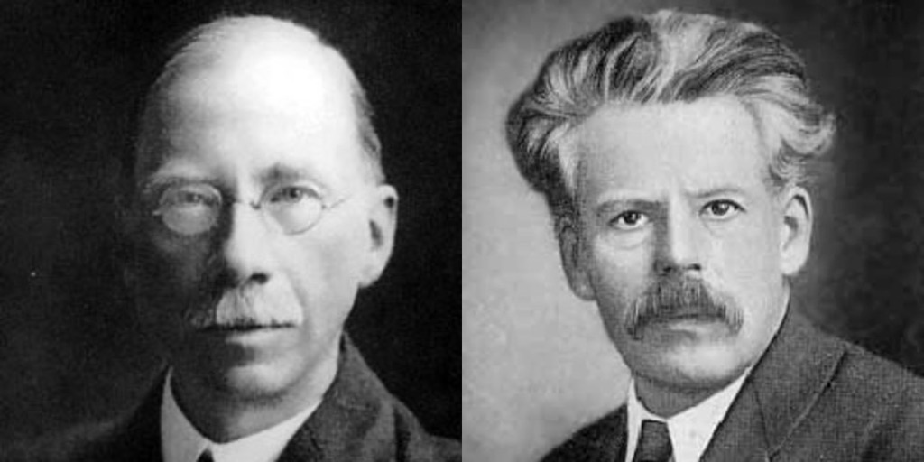
Fig. 5.1 Left: Yule (AR2 model of recurrent business cycles, 1927). Right: Slutsky (moving-average representations of recurrent business cycles, 1927)#
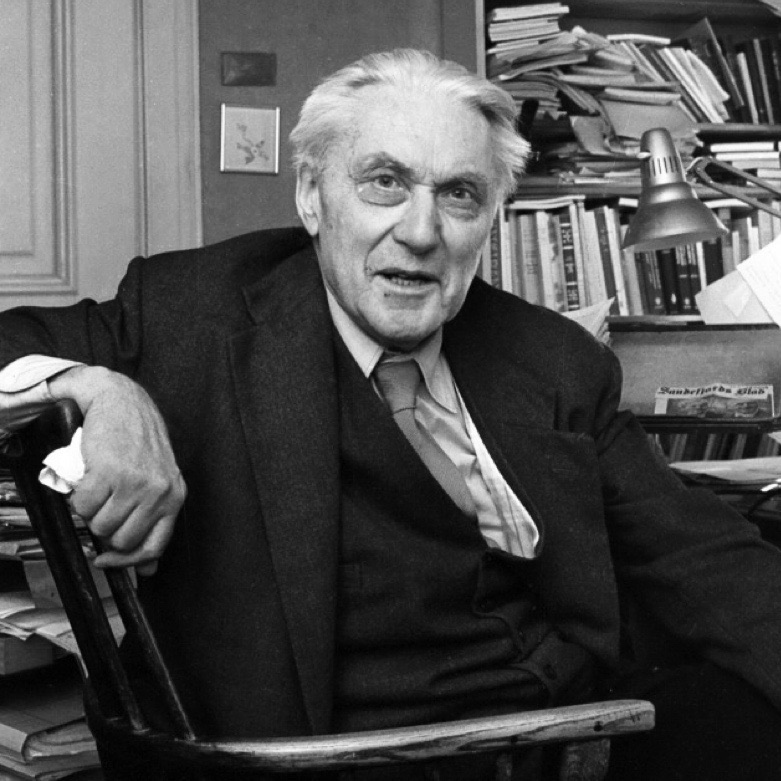
Fig. 5.2 Frisch (Impulse and propagation, 1933)#
“There are alternative ways in which we may approach the impulse problem. … One way which I believe is particularly fruitful and promising is to study what would become of a deterministic dynamic system if it were exposed to a stream of erratic shocks that constantly upsets the continuous evolution, and by so doing introduces in the system the energy necessary to maintain the swings.” – Ragnar Frisch (1933)
5.1. Introduction#
Impulse-response methods have been used by economists since [Frisch, 1933]. Frisch built on earlier insights of [Yule, 1927] and [Slutsky, 1927], who described ways to obtain stochastic recurrent business cycles from linear time series models. Subsequently, [Sims, 1980] showed how to estimate and use vector autoregressive (VAR) systems to model shock transmission across multiple time series. For nonlinear stochastic models, impulse response functions are themselves stochastic processes. In contrast to their linear counterparts, they do not simply scale linearly with increases in the sizes of the impulses. Alternative approaches have been suggested in economics including [Gallant et al., 1993], [Koop et al., 1996], and [Gourieroux and Jasiak, 2005]. This chapter provides stochastic responses in both discrete and continuous time for marginal changes in state variables and shocks. Mathematical support for the continuous-time formulation may be found in [Kunita, 1990], who studies stochastic flows and their pathwise derivatives.
Much, but not all, of the vast literature on VARs treats impulse response functions as ends in themselves. Many applied researchers, for instance, work with what they call “structural VARs” and readily embrace causal language, interpreting identified shocks as exogenous inputs into a dynamical system that “cause” movements in the vector time series of interest. Such impulse response functions are difficult to connect to counterfactuals — the consequences of hypothetical interventions, such as prospective policy changes — which are the purpose of models that are structural in the more classic econometric sense used by builders of dynamic stochastic equilibrium models. See [Marschak, 1953], [Hurwicz, 1966], and [Lucas, 1976] for discussions that link the term structural to policy invariance. On this view, a structural model is one that lets us investigate how a dynamical system changes when one portion of it is altered. When [Hurwicz, 1966] gave a formal definition of a structural model, he chose not to use the term “cause.”
Despite these appropriate reservations about such causal or structural interpretations, the stochastic impulse responses that we characterize in this chapter are key inputs into representing model implications as well as intertemporal marginal valuations. In subsequent chapters, we provide extensive discussions of both types of applications. Chapter 9 constructs what we call shock elasticities that help us characterize the building blocks for exposures to uncertainty and prices of those exposures. These have close connections to the responses featured by [Frisch, 1933], [Sims, 1980] and others in the macroeconomics literature. Chapter 12 provides asset-pricing type representations for the equilibrium valuation of endogenous state variables including various forms of capital. Their use in this context opens the door to dynamic versions of marginal policy assessments as is common in macroeconomics, public finance, and environmental economics.
The responses that we characterize in this chapter are local in nature. They measure how a full vector time series responds to a small change in a state variable or shock at some initial date. They are convenient because they have a simplified structure. In contrast to global calculations for nonlinear models, the local responses scale linearly in the magnitude of the initial perturbation. While they can be suggestive of the impacts of large changes, they are not intended as a substitute for global investigations.
5.2. Discrete time#
We first consider a discrete-time specification.
5.2.1. Markov dynamics#
We start with a Markov process
where there are \(n\) components of the state vector process \(X,\) \(Y\) is a scalar, and \(W\) is a \(k\)-dimensional shock process. We include the \(Y\) process to allow for growth along a common stochastic path. For stochastic equilibrium models, the private sector or policy actions are presumed to be embedded in the dynamic representation.
5.2.2. Discrete-time variational dynamics#
We now construct what we call stochastic responses, although they are sometimes called first variational processes in the applied mathematics literature. We denote by \(\Lambda\) the marginal responses of the \(X\) process, and we denote by \(\Theta\) the marginal responses of the \(Y\) process. Both are stochastic processes. We use the initial conditions, \(\Lambda_0\) and \(\Theta_0,\) to delineate what responses are of interest. For instance, if \(\Lambda_0\) is set to a coordinate vector, we study the responses to a marginal change in the corresponding date-zero state variable, \(X_0\). For these and other initializations, \(({\Lambda_t}^\top, \Theta_t)^\top\) is the date \(t\) state vector stochastic response to the chosen perturbation at the initial date. These variational processes are the stochastic impulse responses to small changes in the underlying state variables.
To obtain a recursive representation for \((\Lambda, \Theta),\) we differentiate (5.1) in a generalized sense to accommodate the stochastic structure and apply the chain rule:
In this calculation, \(\Lambda_{t+1}\) and \(\Theta_{t+1}\) are generally stochastic as they inherit the stochastic dependence of \(X_{t+1}\) and \(Y_{t+1}\) on current and past values of the random shock vector, \(W_{t+1}.\) Moreover, they have the same dimensions as \(X_{t+1}\) and \(Y_{t+1},\) respectively. By differentiating the process at a given initial calendar date, we are allowing for date \(t\) variables to change as a function of date \(t\) information. Not surprisingly, the variational process dynamics depend explicitly on the original state dynamics.
Example 5.1
A sufficient condition for the evolution of the variational processes to be nonstochastic is that
implying that \(\frac{\partial \psi}{\partial x^\top}\) and \(\frac{\partial \kappa}{\partial x}\) are constant. When these derivatives depend on the stochastic state or shock vector, the variational processes are generally stochastic.
Example 5.2
Consider the following quadratic specification:
where \({\mathbb A}_i\) and \({\mathbb D}\) are normalized to be symmetric. This model allows for a form of stochastic volatility as well as quadratic conditional mean dynamics. A simple calculation shows:
This illustrates a specific stochastic structure for the variational processes. As we shall see in Chapter 11, quadratic specifications of this type emerge as second-order approximations to nonlinear stochastic models of state dynamics.
Example 5.3
To obtain responses to initial shocks, set
where we set \(w_0\) to be a coordinate vector with a one in the position corresponding to the particular shock response of interest.
5.3. Continuous-time dynamics#
We now consider the continuous-time counterpart for Brownian motion shocks.
5.3.1. Markov diffusion dynamics#
As a part of a more general derivation, we begin with state dynamics modeled as a Markov diffusion:
where \(W\) is now a \(k\)-dimensional standard Brownian motion. We denote the filtration (intertemporal family of collections of conditioning information events) \({\mathfrak A} \eqdef \left\{ {\mathfrak A}_t : t\ge 0\right\}\) constructed from the Brownian motion and any pertinent date zero information.
5.3.2. Constructing responses#
As in discrete time, we construct the stochastic responses by characterizing the dynamics. As in discrete time, the stochastic responses give the marginal impact on future \(X\) of a marginal change of a particular state or linear combination of states at date zero. Thus we again characterize a process \(\Lambda,\) which has the same number of components as \(X\).
Following the construction in [Kunita, 1990] and [Fournie et al., 1999],
The drift for the \(i^{th}\) component of \(\Lambda\) is
and the coefficient on the Brownian increment is
for \(\lambda\) a hypothetical realization of \(\Lambda_t\) and \(x\) a hypothetical realization of \(X_t.\) Here \(\mu_i\) and \(\sigma_i\) denote the \(i^{th}\) row of the drift vector \(\mu\) and the exposure matrix \(\sigma\) to the Brownian increment, respectively. In particular, \(|\sigma_i|\) is the instantaneous conditional volatility of \(X_t^i\); over an interval \(dt\), the diffusion component has conditional standard deviation \(|\sigma_i|\sqrt{dt}\). The index \(i\) runs over the \(n\) state variables. We isolate the perturbation of interest by our choice of how to initialize \(\Lambda\) at the initial date.[1]
Just as in discrete time, we are led to study the composite process \((X,\Lambda)\) because the Markov evolution of \(\Lambda\) depends on \(X\). Specifically, the composite drift
and the composite matrix coefficient on \(dW_t\) is given by
Let \(\Theta\) be the scalar variational process associated with \(Y.\) Then
Analogous to the discrete-time outcome, the variational dynamics depend explicitly on the original diffusion dynamics.
Example 5.4
Consider the case of linear dynamics, and suppose \({\mathbb A}\) is invertible:
Then
Thus
and
Given the underlying linearity, the global responses follow directly from local responses with a scale adjustment for the size of the increment.
Given the underlying linearity, for this example we have an analytic characterization of the responses and the responses are not stochastic. Our interest is in much more general processes and stochastic evolutions. Even with the absence of analytical solutions, the stochastic responses can be simulated given the underlying state dynamics.
5.3.3. Responses to initial shocks#
So far, we have characterized stochastic responses to initial changes in the state variables. The stochastic responses are formally pathwise derivatives as formalized in [Kunita, 1990]. The responses to shocks can be obtained with alternative initial conditions, although the notion of differentiation is formally different.[2]
In this subsection the index \(i\) runs over the \(k\) shocks rather than the \(n\) states, and \(\sigma_i\) accordingly denotes the \(i^{th}\) column of \(\sigma\) rather than the \(i^{th}\) row as in (5.4); let \(\varsigma_i\) denote the \(i^{th}\) entry of \(\varsigma\), and initialize:
Using these initial conditions, we obtain the continuous-time stochastic responses to shock \(i\) at date zero corresponding to entry \(i\) of \(dW_0\), which we denote \(dW_0^i\). Specifically, the expected impacts of this date-zero shock on \(X\) and \(Y\) are, respectively:
For the special case of linear dynamics given in Example 5.4,
which are the continuous-time counterparts of the familiar impulse responses.
5.3.4. Moving-average representation#
With Markov diffusions, we also have a state-dependent counterpart to a moving-average representation that is well known from linear time series models. The aim is to represent the \(X\) process in terms of the shock contributions at different dates and then “add up” all of the responses across time and components of the Brownian increments.
Stack the shock-specific responses into matrices and vectors:
where \(\Phi_t\) is \(n \times k\) and \(\Psi_t\) is \(1\times k\).
We constructed the processes \(\Phi\) and \(\Psi\) with a date zero initialization. To construct a moving-average representation, we need to shift the date of the initialization. With this in mind, let \({\mathbb S}^u \) be a forward shift operator. When applied to the processes \(\Lambda\) and \(\Theta\), it shifts all of the variables forward, including the initialization date. Note that the Brownian increment, \(dW_u\), induces a stochastic response:
in \(X_t\) and \(Y_t,\) respectively. The stochastic responses include future information. In forming a moving-average representation, we take conditional expectations to eliminate this dependence and then integrate over the shock dates. The resulting formula is known as the Haussmann-Clark-Ocone representation and is given by
When the responses turn out not to be stochastic, as in the case of Example 5.4, the conditional expectations are inconsequential. In this case, we recover the familiar convolution formulas for moving-average representations.
Remark 5.1
Many empirical researchers estimate directly what empirical macroeconomists call local projections, [Jordà, 2005]. These are implemented by regressing a forward sequence of a scalar process on current variables and a shock of particular interest. One can interpret the ambition as wanting to infer impulse responses from direct regressions of future variables on the initial ones. For instance, the aim could be to infer:
by regressing \(X_t\) and \(Y_t\) on a measured shock of interest and including additional variables to purge some of the variation in the measured shock. Some applied papers will include cross terms that are predetermined relative to the shock to accommodate a form of nonlinearity. For this to be coherent, as our analysis makes clear, one has to think through how the nonlinearity compounds within the stochastic system. The shock of interest can alter other variables that in turn influence the variable of interest in future time periods. Our use of variational processes has the advantage that it captures this perspective when the ambition is to measure local impacts.
5.4. Summary#
Stochastic responses \((\Lambda, \Theta)\) are pathwise derivatives of a Markov system with respect to a perturbation at date zero, obtained by differentiating (5.1) and applying the chain rule. They are themselves stochastic whenever the underlying dynamics are nonlinear, and they collapse to conventional impulse responses when \(\psi\) and \(\kappa\) are affine. They are local: they scale linearly in the size of the perturbation, and they are not a substitute for global calculations.
These responses are inputs rather than ends. Chapter 9 uses them to build shock elasticities that separate exposure to uncertainty from the price of that exposure, and Chapter 12 uses them to represent partial derivatives of a value function as asset prices. The chapter also distinguishes these local responses from the causal and structural readings often attached to impulse responses in applied work, a distinction that becomes binding as soon as the responses are used to evaluate hypothetical interventions.
5.5. Exercises#
Exercise 5.1 (Variational dynamics for a quadratic specification)
Example 5.2 states, without derivation, the variational recursions implied by the quadratic state dynamics
where \({\mathbb A}_i\) and \({\mathbb D}\) are symmetric.
(a) Compute the row vector \(\frac {\partial \psi^i}{\partial x^\top}(X_t, W_{t+1})\) for each \(i\), and the row vector \(\frac {\partial \kappa}{\partial x^\top}(X_t, W_{t+1})\).
(b) Apply recursion (5.2) and verify the formulas reported in Example 5.2. Where does the symmetry of \({\mathbb A}_i\) and \({\mathbb D}\) get used?
(c) Which terms in your answer to (a) would have to vanish for the variational processes to be nonstochastic, as in Example 5.1? Which of the constants \({\sf b}_i\) and \({\sf f}\) appear in the variational recursion, and why does their absence make sense?
Exercise 5.2 (Impulse responses of a scalar linear model)
Consider the discrete-time scalar specification
with \(|{\sf a}| < 1\) and \(W_{t+1} \sim {\mathcal N}(0,1)\).
(a) Use recursion (5.2) to write the dynamics of the responses \((\Lambda_t, \Theta_t)\). Explain why they are nonstochastic here, referring to Example 5.1.
(b) For the response to a marginal change in the initial state \(X_0\), set \(\Lambda_0 = 1\) and \(\Theta_0 = 0\). Solve for \(\Lambda_t\) and \(\Theta_t\), and report their limits as \(t \rightarrow \infty\).
(c) For the response to a marginal date-zero shock, initialize instead with \(\Lambda_0 = \frac{\partial \psi}{\partial w}(X_0, 0) = {\sf b}\) and \(\Theta_0 = \frac{\partial \kappa}{\partial w}(X_0, 0) = {\sf f}\). Solve for \(\Lambda_t\) and \(\Theta_t\) and interpret them as impulse responses.
(d) Example 9.1 of Chapter 9 computes a shock elasticity for the multiplicative functional \(M = \exp(Y)\) built from this same system. Specialized to the scalar case with \(\pi = 1\), that formula reads
Compare it with your \(\Theta_t\) from (c). What exactly is the relation, and why should a derivative with respect to the size of a date-one exposure to uncertainty agree with a cumulative response to a date-zero state perturbation? Then let \(t \rightarrow \infty\) in both and identify the common limit as an object from Chapter 3 and Chapter 4.
Exercise 5.3 (A continuous-time Ornstein-Uhlenbeck example)
Consider the scalar diffusion
with \(\theta > 0\) and \(W\) a scalar standard Brownian motion.
(a) Identify \({\mathbb A}, {\mathbb B}, {\mathbb D}, {\mathbb F}\) in the notation of Example 5.4, check that \({\mathbb A}\) is invertible, and write the composite drift (5.3) and exposure matrix (5.4).
(b) Solve for the state response \(\Lambda_t\) given \(\Lambda_0\) and, with \(\Theta_0 = 0\), for \(\Theta_t\).
(c) Compute the responses of \(X\) and \(Y\) to a date-zero Brownian shock by initializing \(\Lambda_0 = \sigma\) and \(\Theta_0 = \varsigma = 0\). Interpret the limits as \(t \rightarrow \infty\).
Exercise 5.4 (When responses become stochastic)
Now let the state evolve nonlinearly,
a scalar instance of Example 5.2.
(a) Write the variational recursion for \(\Lambda_t\) and \(\Theta_t\).
(b) With \(\Lambda_0 = 1\), solve for \(\Lambda_t\) as a product, and explain why it is a stochastic process, in contrast to Exercise 5.2.
(c) Show that the conditional-mean response \({\mathbb E}\left( \Lambda_t \mid X_0 \right)\) is generally not equal to the linear benchmark \({\sf a}^t\). Compute it for \(t = 1\) and \(t = 2\).
(d) Remark 5.1 observes that some applied papers add cross terms to a local projection to accommodate nonlinearity. Using your answer to (c), explain what such a regression would have to reproduce in order to recover \({\mathbb E}\left( \Lambda_2 \mid X_0 \right)\).
5.6. Answers#
Solution to Exercise 5.1 (Variational dynamics for a quadratic specification)
(a) Differentiating the \(i^{th}\) equation with respect to \(x\) and writing the result as a row vector,
where the middle term uses \(\frac{\partial}{\partial x}\left({\frac 1 2} x^\top {\mathbb A}_i x \right) = {\mathbb A}_i x\) for symmetric \({\mathbb A}_i\). Similarly,
(b) Post-multiplying by \(\Lambda_t\) as recursion (5.2) requires,
Each of the last two terms is a scalar and so equals its own transpose: \({X_t}^\top {\mathbb A}_i \Lambda_t = {\Lambda_t}^\top {{\mathbb A}_i}^\top X_t = {\Lambda_t}^\top {\mathbb A}_i X_t\), where the second equality is where symmetry of \({\mathbb A}_i\) is used, and \({W_{t+1}}^\top {{\mathbb B}_i}^\top \Lambda_t = {\Lambda_t}^\top {\mathbb B}_i W_{t+1}\). This reproduces
The same steps applied to \(\kappa\), using symmetry of \({\mathbb D}\), give
as reported in Example 5.2.
(c) The responses are nonstochastic when the derivatives in (a) do not depend on \(X_t\) or \(W_{t+1}\), which requires \({\mathbb A}_i = 0\) and \({\mathbb B}_i = 0\) for every \(i\), and \({\mathbb D} = 0\) and \({\mathbb F} = 0\). What survives is the affine case \({\sf a}_i \cdot X_t + {\sf b}_i \cdot W_{t+1}\) flagged in Example 5.1.
The constants \({\sf b}_i\) and \({\sf f}\) do not appear in the variational recursion at all. They multiply \(W_{t+1}\) alone, so they drop out on differentiation with respect to \(x\). This is as it should be: \({\sf b}_i \cdot W_{t+1}\) is the part of next period’s state that a marginal change in today’s state cannot affect. Those constants do reappear if instead we perturb the date-zero shock, since they then enter through the initialization of \(\Lambda_0\) and \(\Theta_0\).
Solution to Exercise 5.2 (Impulse responses of a scalar linear model)
(a) Since \(\psi(x,w) = {\sf a} x + {\sf b} w\) and \(\kappa(x,w) = \nu + {\sf d} x + {\sf f} w\), we have \(\frac{\partial \psi}{\partial x} = {\sf a}\) and \(\frac{\partial \kappa}{\partial x} = {\sf d}\). Recursion (5.2) becomes
Both derivatives are constants, so the responses do not depend on the realized shocks; this is the affine case flagged in Example 5.1.
(b) With \(\Lambda_0 = 1\), iterating gives \(\Lambda_t = {\sf a}^t\). Summing the increments of \(\Theta\) from \(\Theta_0 = 0\),
As \(t \rightarrow \infty\), \(\Lambda_t \rightarrow 0\) (the state response dies out) and \(\Theta_t \rightarrow \frac{\sf d}{1 - {\sf a}}\) (the cumulative response of \(Y\) settles at a finite level).
(c) The recursion is unchanged, so \(\Lambda_t = {\sf a}^t \Lambda_0 = {\sf a}^t {\sf b}\) and
Here \(\Lambda_t = {\sf a}^t {\sf b}\) is the moving-average coefficient giving the response of \(X_{t}\) to a unit date-zero shock, while \(\Theta_t\) accumulates the responses of \(Y\), approaching \( {\sf f} + \frac{{\sf d}\,{\sf b}}{1 - {\sf a}}\) as \(t \rightarrow \infty\). These are the familiar impulse responses of a linear time-series model.
(d) They are the same sequence, shifted by one period: \(\epsilon^m(x,t) = \Theta_{t-1}\) at every horizon, exactly.
The reason is that both quantities pick off the same coefficient. Write \(Y_t - Y_0 = {\sf const} + \sum_{j=1}^t c_j W_j\) and solve for the loading on \(W_j\):
The perturbation used in Chapter 9 tilts the mean of \(W_1\), and because \(M\) is log-normal here the elasticity extracts precisely \(c_1\). Part (c) accumulates the response of \(Y\) to a shock, reaching \(\Theta_{t-1} = c_1\) after \(t-1\) steps. The one-period shift is a timing convention: the elasticity perturbs at date one, the response at date zero.
The agreement is special to this specification. Part (a) established that the responses here are nonstochastic, so a marginal change in exposure to a shock and a marginal change in the state propagate through identical constant coefficients. Once \(\frac{\partial\psi}{\partial x}\) or the conditional volatility depends on the state, the two calculations separate: responses stay derivatives with respect to a state, elasticities become derivatives with respect to an exposure, and only the latter carries the change of measure that Chapter 9 uses at long horizons.
Both limits are
which is the scalar case of \({\mathbb F} + {\mathbb D}({\mathbb I}-{\mathbb A})^{-1}{\mathbb B}\) in (4.6) of Chapter 4: the coefficient on the permanent shock, equivalently \(\alpha(1)\) of Section Permanent shocks of Chapter 3. A shock’s long-run effect on the level of \(Y\), its limiting shock elasticity, and the martingale increment extracted from \(Y\) are three descriptions of one number.
Solution to Exercise 5.3 (A continuous-time Ornstein-Uhlenbeck example)
(a) Matching \(\mu(x) = {\mathbb A} x\), \(\sigma(x) = {\mathbb B}\), \(\nu(x) = {\mathbb D} x\), \(\varsigma(x) = {\mathbb F}\) gives \({\mathbb A} = -\theta\), \({\mathbb B} = \sigma\), \({\mathbb D} = 1\), and \({\mathbb F} = 0\). Since \(\theta > 0\), \({\mathbb A} = -\theta \neq 0\) is invertible, as Example 5.4 requires. Because \(\mu\) is linear and \(\sigma\) is constant,
so \(d\Lambda_t = -\theta \Lambda_t\, dt\), which is nonstochastic, and \(d\Theta_t = \Lambda_t\, dt\).
(b) From Example 5.4, \(\Lambda_t = \exp(-\theta t)\, \Lambda_0\) and
(c) With \(\Lambda_0 = \sigma\) and \(\Theta_0 = 0\),
The response of \(X\) to the shock decays at rate \(\theta\) back to zero, which is mean reversion, while the response of \(Y\) builds up monotonically to the permanent level \(\sigma / \theta\). The responses are nonstochastic because the dynamics are linear with a constant exposure to the Brownian increment.
Solution to Exercise 5.4 (When responses become stochastic)
(a) Here \(\frac{\partial \psi}{\partial x} = {\sf a} + \alpha X_t\) and \(\frac{\partial \kappa}{\partial x} = {\sf d}\), so
(b) Iterating from \(\Lambda_0 = 1\),
The multiplier \({\sf a} + \alpha X_s\) now depends on the realized state \(X_s\), which is random, so \(\Lambda_t\) is a stochastic process — the phenomenon anticipated in Example 5.1, where variational processes are stochastic precisely when \(\frac{\partial \psi}{\partial x}\) is not constant. When \(\alpha = 0\) we recover the deterministic \(\Lambda_t = {\sf a}^t\) of Exercise 5.2.
(c) Because \(\Lambda_t\) covaries with the state path, its conditional mean is state dependent. Since \(\Lambda_1 = {\sf a} + \alpha X_0\) is known at date zero,
which already differs from \({\sf a}\) unless \(\alpha = 0\). For \(t = 2\), use the Law of Iterated Expectations together with \({\mathbb E}\left( X_1 \mid X_0 \right) = {\sf a} X_0 + {\frac 1 2}\alpha X_0^2\) to obtain
The mean impulse response depends on the initial state \(X_0\) and is not \({\sf a}^t\); nonlinear responses do not simply reproduce their linear counterparts.
(d) The answer to (c) is a quadratic function of \(X_0\), and its coefficients are particular products of \({\sf a}\) and \(\alpha\) rather than free parameters. A local projection that regresses \(X_2\) on the date-zero shock interacted with \(X_0\) could in principle fit a linear term in \(X_0\), but to recover \({\mathbb E}\left( \Lambda_2 \mid X_0 \right)\) it would also need the \(X_0^2\) term, and at horizon \(t\) it would need a polynomial of degree \(t\). The order of the interaction that a projection requires therefore grows with the horizon, and the coefficients across horizons are restricted by the single pair \(({\sf a}, \alpha)\). As Remark 5.1 puts it, one has to think through how the nonlinearity compounds within the stochastic system.