
11. Using Recursive Utility to Assess Uncertainty#
Authors: Jaroslav Borovicka (NYU), Lars Peter Hansen (University of Chicago), and Thomas J. Sargent (NYU)
\(\newcommand{\eqdef}{\stackrel{\text{def}}{=}}\)

“Uncertainty is the only certainty there is, and knowing how to live with insecurity is the only security.” - John Allen Paulos
11.1. Introduction#
This chapter studies the recursive utility preference specification of [Kreps and Porteus, 1978] and [Epstein and Zin, 1989]. We include interpretations of this specification proposed by [Hansen and Sargent, 2001] and [Anderson et al., 2003] that are designed to capture concerns about model misspecification. We deploy two distinct approximation approaches. One approach builds on a characterization by [Duffie and Epstein, 1992] and uses a continuous-time limiting approximation to a discrete-time specification in which underlying shocks are normally distributed. Our account of the approximation differs in details from that of [Duffie and Epstein, 1992]. We represent the limiting approximation with a Brownian motion information structure. Our second approximation lets macroeconomic uncertainty have first-order consequences. We modify first- and second-order approximations routinely used in the macroeconomics literature in ways designed to focus on macroeconomic uncertainty and explore implications of (nonstandard) first- and second-order approximations to equilibria of dynamic stochastic models. Our approximations apply to production-based macro-finance models in which there are opportunities to invest in different kinds of capital. Our approximation approaches use a change in probability measure to represent a decision maker’s adjustments for uncertainty. We shall see that this adjustment differs from the one underlying the so-called risk neutral distribution that is widely used to price derivative claims. Our change of measure instead emerges from specifications of preferences like those in [Hansen and Sargent, 2001] and [Anderson et al., 2003] that build on a robust control literature initiated by [Jacobson, 1973] and [Whittle, 1981].
We extend work by [Schmitt-Grohé and Uribe, 2004] and [Lombardo and Uhlig, 2018] in ways that highlight consequences of uncertainty. We design approximations to make implied stochastic discount factors reside within an exponential linear quadratic class, a class that gives rise to tractable formulas for asset valuation over alternative investment horizons. See, for instance, [Ang and Piazzesi, 2003] and [Borovička and Hansen, 2014]. The class is also useful for studying production-based macro-finance models with opportunities to invest in different forms of capital.
Note
We recognize that nonlinearities can be more accurately captured by global solution methods. Sometimes these are too costly or just not feasible.
11.2. Recursive utility valuation process#
We construct continuation value and stochastic discount processes, important constituents of many dynamic stochastic models in macroeconomics and finance.
11.2.1. Basic recursion#
A homogeneous degree-one representation of recursive utility is
where
Value \(V_t\) defined in equation (11.1) is a homogeneous of degree one function of \(C_t\) and \(R_t\); equation (11.2) defines \(R_t\) as a homogeneous of degree one function of another function of \(V_{t+1}\).
In equation (11.1), \(0 < \beta < 1\) is a subjective discount factor and \({\frac 1 \rho}\) is the elasticity of intertemporal substitution, while \(\gamma\) in equation (11.2) describes attitudes towards risk. Section An economic rationale of Chapter 4 worked through the \(\rho = 1\) special case of these recursions for a first-order vector autoregression; this chapter treats general \(\rho\) and shows how to approximate the resulting objects.
Continuation values are determined only up to an increasing transformation. For computational and conceptual reasons, it is useful to work with the transformation \({\widehat V}_t = \log V_t\). Recursions for \({\widehat V}_t\) expressed in terms of the logarithm of consumption \({\widehat C}_t\) are
where
The right side of recursion (11.3) is the logarithm of a constant elasticity of substitution (CES) function of \(\exp({\widehat C}_t)\) and \(\exp({\widehat R}_t)\).
Remark 11.1
The limit of \({\widehat R}_t\) as \(\gamma\) approaches \(1\) is expected logarithmic utility:
We shall construct small noise expansions of \({\widehat V}_t\) and \({\widehat R}_t\) separately, then assemble them. Before doing so, we offer a reinterpretation of our recursions (11.3)-(11.4).
11.2.2. Preference for robustness#
When \(\gamma > 1\), (11.4) emerges as an indirect utility function for a robust control problem in which \(\frac 1 {\gamma - 1}\) serves as a penalty parameter on entropy of an alternative model relative to a baseline model.
The interpretation of (11.4) as an indirect utility function from a minimization problem originated in [Hansen and Sargent, 1995], which rested on earlier work by [Jacobson, 1973] and [Whittle, 1981]. Chapter 10 provides the decision-theoretic foundations for this construction and situates it within a family of divergence-penalized preferences.
Let the random variable \(N_{t+1} \ge 0\) satisfy \({\mathbb E} \left( N_{t+1} \mid {\mathfrak A}_t \right) = 1\) so that it is a likelihood ratio. Think of replacing the expected continuation value \({\mathbb E} \left( {\widehat V}_{t+1} \mid {\mathfrak A}_t \right)\) by
where \(\xi\) is a parameter that penalizes departures of \(N_{t+1}\) from unity as measured by relative entropy. Conditional entropy relative to an alternative conditional probability induced by applying a change of measure \(N_{t+1}\) is
which, because \(n \log n\) is a convex function, follows from Jensen’s inequality. Evidently, this inequality becomes an equality when \(N_{t+1} = 1\).
Relative entropy serves as a summary measure of the difference between two probability distributions. We can think of \(N_{t+1}\) as a conditional likelihood ratio of an alternative model relative to a baseline model. Then \({\mathbb E} \left( N_{t+1} \log N_{t+1} \mid {\mathfrak A}_t \right)\) is an expected (conditional) log-likelihood ratio of the alternative model when the expectation is taken using the alternative probability model. A small expected log-likelihood ratio indicates a small discrepancy between two models, i.e., two probability distributions.
Remark 11.2
To solve minimization problem (11.5), attach a Lagrange multiplier \(\ell\) to the constraint and form a Lagrangian. Then minimize with respect to the random variable \(N\) and maximize it with respect to \(\ell\). This extremization problem separates across states, so to minimize with respect to \(N\) we can solve the following minimum problem for each possible \(n\)
Here \(n\) is a potential realization of \(N_{t+1}\) and \({\hat v}\) is a potential realization of \({\widehat V}_{t+1}.\) First-order necessary conditions are:
which implies the minimizer
and the minimized objective
To determine \(\ell,\) we pose
whose first-order necessary condition is
The maximizing \(\ell\) is
and the minimized objective function is
The minimizing \(N_{t+1}\) is
The minimizer (11.6) of problem (11.5) evidently shifts probabilities toward low continuation values, so that probabilities of undesirable events are raised and probabilities of desirable events are lowered. [Bucklew, 2004] called this a stochastic version of Murphy’s law. Notice that the minimized objective satisfies
where earlier we described \({\widehat R}_t\) by equation (11.4) after we set \(\xi = {\frac 1 {\gamma - 1}} \).
It follows from (11.6) that
The random variable \(N_{t+1}^*\) will appear often below.
11.2.3. Stochastic discount factor process#
A stochastic discount factor (SDF) process \(S = \{ S_t : t \ge 0 \}\) describes a consumer’s attitudes about small changes in uncertainty. SDF processes have several uses. First, they contain shadow prices that tell how a consumer’s attitudes about uncertainty shape marginal valuations of risky assets. Second, they shape first-order necessary conditions for optimally choosing financial and physical investments. Third, they underlie tractable formulas for equilibrium asset prices. Fourth, they can help construct Pigouvian taxes that ameliorate externalities under uncertainty. Fifth, they can help evaluate effects of small (local) changes in government policies.
To deduce an SDF process, we posit that a date zero value of a risky date \(t\) consumption payout \(\chi_t\) is
To compute the ratio \( \frac {S_t}{S_0} \) that appears in formula (11.7) we evaluate the slope of an indifference curve that connects a baseline consumption process \(\{C_t\}_{t=0}^\infty\) to a perturbed consumption process
The scalar \({\sf q}\) parameterizes an indifference curve; \(P_0({\sf q})\) is the reduction in current consumption that keeps a consumer on that curve after we replace \(C_t\) by \(C_t + {\sf q} \chi_t\). We set \(\pi_0^t(\chi_t)\) defined in equation (11.7) equal to the slope of that indifference curve:
For recursive utility, a one-period increment in the stochastic discount factor process is
where
and \(N_{t+1}^*\) induces the change of probability measure that equation (11.6) presents as the outcome of a robust valuation problem. By design, the construction of \({\widehat S}_{t+1} - {\widehat S}_t\) captures the terms involving \(\rho\). We will use the second line in (11.8) in what follows. We will think of \(\beta\) as a subjective discount factor adjustment, \(N_{t+1}^*\) as a change-of-measure adjustment for uncertainty, and \(\exp\left({\widehat S}_{t+1} - {\widehat S}_t \right)\) as an adjustment for the elasticity of intertemporal substitution. We interpret the twisted transition probability measure induced by \(N_{t+1}^*\) as an adjustment for uncertainty about evaluations.
The recursive structure of preferences makes the time-\(t\) stochastic discount factor \(\frac {S_t}{S_0}\) the product of the respective one-period stochastic discount factor increments. Similarly, we can compound one-period transition uncertainty measures into multiple time-horizon measures of uncertainty.
Remark 11.3
To verify formula (11.8), we compute a one-period intertemporal marginal rate of substitution. Given the valuation recursions (11.3) and (11.4), we construct two marginal utilities, one each for CES and exponential one-period utility functions:
From the certainty equivalent formula, we construct the marginal utility of the next-period logarithm of the continuation value:
where the \(+\) superscript is used to denote the next-period counterpart. The next-period marginal utility of consumption is
Putting these four formulas together using the chain rule for differentiation gives a marginal rate of substitution:
Now let \({\hat v}^+ = {\widehat V}_{t+1}\), \(c^+ = C_{t+1}\), \(c = C_t\), and \({\hat r} = {\widehat R}_t\) to obtain the formula for the one-period stochastic discount factor (11.8).
11.3. Continuous-time limit#
We now study a continuous-time limit that approximates a discrete-time specification. Since we continue to work with normal shocks, the continuous-time counterparts are Brownian increments. The continuation value in continuous time will evolve as:
for some drift (local mean), \(V_t \mu_t^V\) and some local shock exposure vector \(V_t \sigma_t^V\), where \(\{W_t : t \ge 0\}\) is a multivariate Brownian motion. Scaling the local evolution coefficients by \(V_t\) is convenient when the continuation value process is presumed to be positive. As in discrete time, it is convenient to work with the logarithm of the continuation value process (the log is a strictly increasing transformation). The implied evolution is
where \({\hat \mu}_t^V = {\mu}_t^V - {\frac 1 2} \mid \sigma_t^V \mid^2.\) This adjustment follows from Ito’s formula.
11.3.1. Discrete-time approximation#
To study the utility recursion, start with a discrete-time specification:
where \(\beta_\epsilon = \exp(- \delta \epsilon)\) and \(\delta>0\) is the instantaneous subjective rate of discount. Consider the time derivative of the second recursion:
by local log normality.
We turn now to the first recursion and compute time derivatives in three steps. First, we evaluate the term inside the logarithm as \(\epsilon\) tends to zero:
This term is in the denominator as implied by the derivative with respect to a logarithm. Second, we differentiate the term inside the logarithm with respect to \(\epsilon\) as contributed by \(\beta_\epsilon\):
Third, we differentiate the term inside the logarithm with respect to \(\epsilon\) as contributed by
Putting together the derivative components gives:
This relation imposes a restriction across the local mean \({\mu}_t^V\) and the local variance \( |\sigma_t^V|^2\) of the continuation value. [Duffie and Epstein, 1992] refer to \(\gamma\) as a variance multiplier where larger values of \(\gamma\) imply a more substantial adjustment for local volatility. As in discrete time, the \(\rho = 1\) case is an interesting special case represented as:
11.3.2. Robustness to misspecification#
To investigate an aversion to model misspecification in continuous time, we now treat the distribution of \(\{W_t : t\ge0\}\) as uncertain. We allow for probability measures that entertain possible Brownian motions with local means or drifts that are history dependent.
We start by considering positive martingales \(\{ M^H_t : t \ge 0\}\) parameterized by
alternative \(\{ H_t : t \ge 0\}\) processes with the same dimension as the underlying Brownian motion.
The martingales have local evolutions:
and we initialize them at \(M_0^H = 1\). Observe that by applying Ito’s formula, \(\log M^H\) evolves as:
We use these martingales as relative densities or likelihood ratios.
Write the discrete-time counterpart as
Let \(w\) be a realized \(W_{t+\epsilon} - W_t\) and \(h\) be a realization of \(H_t\). Then \(\log M_{t+\epsilon} - \log M_t\) contributes \( -{\frac \epsilon 2}h'h + h\cdot w \) to the log-likelihood. Writing \(d\) for the dimension of the Brownian motion, the density of \(W_{t+\epsilon} -W_t\), which is normal with mean zero and covariance matrix \(\epsilon I\), contributes \(-{\frac 1 {2\epsilon}} w'w - {\frac d 2}\log (2 \pi \epsilon)\). Putting these two components together, we have a log-likelihood:
The altered conditional density has mean \(\epsilon h\), which is the realized value of \(\epsilon H_t\) with the same conditional covariance matrix as before. Moreover, the conditional expectation of
which measures the statistical divergence or relative entropy between original and altered conditional probabilities.
For the continuous-time limit, under the \(H\) change of probability measure:
where \({\widetilde W}^H\) is a standard Brownian motion. Thus, potential changes of probability measures induce local means or drift \(H\) processes to the Brownian motion. The continuous-time counterpart to conditional relative entropy at time \(t\) is \({\frac 1 2} \left| H_t \right|^2.\)
We can justify focusing on drift distortions for Brownian increments because of our imposition of absolute continuity of the alternative probabilities with respect to the baseline specification of a multivariate standard Brownian motion. This is an implication of the Girsanov Theorem.
We can now deduce a robustness adjustment in continuous time. Consider formula (11.10) when \(\gamma = 1\) modified for a potential change in the probability measure
Modify this equation to include minimization over \(H_t\) subject to a relative entropy penalty \(\frac \xi 2 |H_t|^2:\)
The minimizer is
with a minimized objective
Notice that this agrees with formula (11.10) for \(\gamma - 1= 1/\xi\). The explicit link is entirely consistent with our discrete-time equivalence result. By taking the continuous-time limit, we are able to focus our misspecification analysis on changing local means of the underlying Brownian increments.
11.3.3. Uncertainty pricing#
To prepare the way for studying valuations, we compound the equilibrium version of \(\{ H_t^* : t \ge 0\}\) to get an exponential martingale:
provided that the constructed process is a martingale.[1] With this construction we interpret \(-H_t^*\) as the vector of local uncertainty prices that give compensations for exposure to Brownian increment uncertainty. These compensations are expressed as changes in conditional means under the baseline distribution, as is typical in continuous-time asset pricing.
Example 11.1
We explore a robust counterpart to the [Borovička, 2020] model we introduced in Example 8.4. This model has two investor types, each with a different set of baseline beliefs. In what follows, we let superscripts index the individuals and we include parentheses when we raise variables to powers. The economic environment is as follows.
Preferences
The investor types have the same subjective rate of discount, \(\delta\) and the same unitary elasticity of intertemporal substitution. [Borovička, 2020] does not impose the latter restriction and formulates a planner’s problem with a different endogenous state.
Beliefs
Investor \(n\) believes the exogenously specified aggregate state of the economy evolves as:
\[d \log Y_t = (\mu_y + \sigma_y u^n) dt + \sigma_y dW_t^n\]where \(W^n\) is a standard Brownian motion under the baseline beliefs of person \(n\).
Consumption
Output is split into consumption allocated between the two investor types. Let \(\zeta^n = C^n / Y\), where \(C^n\) is the consumption of investor \(n\). Then
Robustness concerns
The subjective beliefs in conjunction with an \(H\) process used to capture robust adjustments are multiplicative martingales with logarithms that evolve as:
\[d \log M_t^n = -\frac{(H_t^n + u^n)^2}{2} dt + (H_t^n + u^n)dW_t^{H^n}\]for \(n=1,2.\) We let \(\xi^n\) denote the penalty parameters used to limit the robustness explorations.
We compute competitive equilibria using a planner’s problem with an endogenous state variable process
\[X_t = \log M_t^2 - \log M_t^1.\]Our approach is an extension of one proposed by [Negishi, 1960]. Alternative competitive equilibrium allocations correspond to alternative initializations of the two martingales, obtained by solving a robust version of a planner’s problem. Write the stochastic evolution for \(X\) under the baseline probabilities as:
\[dX_t = \mu_x(X_t) dt + \sigma_x(X_t) dW_t\]where formulas for \(\mu_x\) and \(\sigma_x\) are given in the Appendix to this chapter.
Value function construction for a robust planner
Write \(y\) for a realization of \(\log Y_t\), \(m^n\) for a realization of \(M_t^n\), and \(x\) for a realization of \(X_t\). Guess a planner value function of the form:
\[(m^1 + m^2)y + m^1 v(x) .\]Construct the planner HJB equation:
\[\begin{split}\begin{split} 0 =& \max_{\zeta^1, \zeta^2, \zeta^1 + \zeta^2 = 1} \min_{h^1, h^2} -\delta v + \delta \log(\zeta^1) + \delta \exp(x)\log(\zeta^2) \\ &+ \frac{dv}{dx}\left[ \mu_x + \sigma_x \left(h^1 + u^1\right) \right] + \frac{d^2 v}{dx^2} \frac {\sigma_x^2} 2\\ & + \left[\mu_y + \sigma_y(h^1 + u^1)\right] + \exp(x)\left[\mu_y + \sigma_y(h^2 + u^2)\right] \\ &+ \xi^1 \frac{(h^1)^2}{2} + \exp(x)\xi^2\frac{(h^2)^2}{2}. \end{split}\end{split}\](where we divided through by \(m^1\)). Importantly, the robust planner solves a max-min problem where the minimization includes the possibility of distinct drift distortions for each of the investor types.
The figure that follows gives an interactive characterization of alternative equilibria. The sliders set the optimistic investor’s belief parameter \(u^2\) and the robustness penalty parameters \(\xi^1\) and \(\xi^2.\) For some specifications, there will not be a stationary density for the underlying endogenous state variable. The consumption fraction, \(\zeta^n\), allocated to the type \(n\) of investors is monotone in the endogenous state variable. The first two plots give the implied drift distortions for the aggregate consumption dynamics
expressed as a function of the corresponding consumption \(\zeta^n.\)
The next two plots depict the stationary densities for \(\zeta^1\) and \(\zeta^2\) under the benchmark probability specification, when in fact such a density exists.
As is shown in the Appendix, the Chernoff entropy calculations are the same for \(n=1,2\). The fifth plot shows the asymptotic decay rate for each \(0<\alpha<1\) and reports its maximum as the Chernoff entropy, denoted \(\eta^*.\) We also report
which is an equivalent constant drift distortion with the same Chernoff entropy. This provides an alternative perspective on the magnitude of this entropy. An interesting set of experiments is to set \(u^2 = .25,\) \(\xi^2 = 1/3\), and to consider \(\xi^1 = 1/4, 1/5, ... , 1/12.\) The Chernoff entropy increases as we make the investors with correct beliefs less confident in the baseline probability specification. At the same time, the stationary densities for the consumption fractions overlap more as we reduce this confidence. As an alternative, when we fix \(\xi^1 = 1/3\) and let \(\xi^2 = 1/4, 1/5, ... , 1/12,\) the Chernoff entropies are decreasing as we make the optimistic investor less confident in the baseline specification. The Chernoff calculation does not converge when we set \(\xi^1 = \xi^2 = 1/3\) and \(u^2 = .25.\)
In a model comparison paper, [Hansen et al., 2024] use a continuous-time specification as we described here and discuss the continuous-time methods for shock elasticities as barometers for the alternative models. The models include ones with two capital stocks differentially exposed to uncertainty and ones with two types of agents differentially exposed to financing constraints.
11.4. Small noise expansion of dynamic stochastic equilibria#
We now study another characterization that sometimes helps provide good approximations of equilibria of dynamic stochastic models.[2] In Section A quadratic approximation of state dynamics of Chapter 4 we described a pathwise approximation for a process with stationary Markov increments following on previous research by [Lombardo and Uhlig, 2018]. We now use that approximation as a central input into a model solution building on the [Lombardo and Uhlig, 2018] approach, but we extend it in a way that emphasizes uncertainty impacts even in first-order contributions. This outcome is in contrast to previous treatments of second-order approximations given, for instance, in [Schmitt-Grohé and Uribe, 2004]. By design, our approximations of stochastic discount factors reside within the exponential linear quadratic class, a class known to provide tractable formulas for asset valuations across investment horizons. See, for instance, [Ang and Piazzesi, 2003] and [Borovička and Hansen, 2014]. Furthermore, these approximations apply to production-based macro-finance models with investment opportunities in alternative types of capital.
While these approximations are tractable, we recognize that they might omit or disguise important aspects of uncertainty. Without question, global solution methods capture important nonlinearities more accurately for some models. Nevertheless, the approximations to be presented here shed light on the structures of preferences and their implications for asset pricing in both endowment and production economies.
11.4.1. Approximate state dynamics#
We start by following [Lombardo and Uhlig, 2018] and considering the class of stochastic processes indexed by a scalar perturbation parameter \(\mathsf{q}\):[3]
Following Section A quadratic approximation of state dynamics of Chapter 4, let \(X\) be an \(n\)-dimensional stochastic process and let \(\{W_{t+1}\}\) be an i.i.d. sequence of normally distributed random vectors with conditional mean vector \(0\) and conditional covariance matrix \(I\). We parameterize this family so that \({\sf q} = 1\) gives the model of interest.
We denote the zero-order expansion \({\sf q} = 0\) limit as:
and assume that there exists a second-order expansion of \(X_{t}\) around \(\mathsf{q} = 0\):
where \(X_t^1\) is a first-order contribution and \(X_t^2\) is a second-order contribution. The processes \(X^1\) and \(X^2\) are the first and second derivatives of \(X\) with respect to the perturbation parameter \({\sf q}\), evaluated at \({\sf q} = 0\).
In the remainder of this chapter, we shall construct instances of the second-order expansion (11.13) in which the generic random variable \(X_t\) is replaced, for example, by the logarithm of consumption, a value function, and so on.
Processes \(X_t^j, j=0, 1, 2\) have a recursive structure: first compute the stochastic process \(X_{t}^0,\) then the process \(X_{t}^1\) (it depends on \(X_t^0\)), and finally the process \(X_{t}^2\) (it depends on both \(X_{t}^0\) and \(X_{t}^1\)).
Remark 11.4
Perturbation methods have been applied to many rational expectations models in which partial derivatives of \( \psi \) with respect to \(\mathsf{q}\) are often zero.[4] However, derivatives of \( \psi \) with respect to \(\mathsf{q}\) are not zero in production-based equilibrium models with the robust or recursive utility specifications that we shall study here.
Let \(C\) denote consumption and \({\widehat C}\) the logarithm of consumption. Following Section A quadratic approximation of state dynamics of Chapter 4, suppose that the logarithm of consumption evolves as:
Approximate this process by:
In models with endogenous investment and savings, consumption dynamics as well as some of the state dynamics emerge as equilibrium outcomes. We use the approximating processes (11.13) and (11.14) as inputs for constructing an approximate continuation value process and its risk-adjusted counterpart under recursive utility preferences.
11.5. Incorporating preferences with enhanced uncertainty concerns#
To approximate the recursive utility process, we deviate from common practice in macroeconomics by letting the risk aversion or robustness parameters in preferences depend on \({\sf q}\):
The aversion to model misspecification or the aversion to risk moves inversely with the parameter \({\sf q}\) when we embed the model of interest within a parameterized family of models. In effect, the variable \({\sf q}\) is doing double duty. Reducing \({\sf q} > 0\) limits the overall exposure of the economy to the underlying shocks. This is offset by letting the preferences include a greater aversion to uncertainty. This choice of expansion protocol has significant and enlightening consequences for continuation value processes and for the minimizing \(N\) process used to alter expectations. It allows for limiting behavior that expresses uncertainty implications at lower orders of approximation. It has antecedents in the control theory literature, and it has the virtue that implied uncertainty adjustments occur more prominently at lower-order terms in the approximation.
11.5.1. Order-zero#
Write the order-zero expansion of (11.3) as
where the second equation follows from noting that randomness vanishes in the limit as \(\mathsf{q}\) approaches \(0\).
For order zero, write the consumption growth-rate process as
The order-zero approximation of (11.3) is:
We guess that \({\widehat V}_t^0 - {\widehat C}_t^0 = \eta_{v-c}^0\) and will have verified the guess once we solve:
This equation implies
Equation (11.15) determines \( \eta_{v - c}^0\) as a function of \(\eta_c^0\) and the preference parameters \(\rho, \beta\), but not the risk aversion parameter \(\gamma\) or its robust counterpart \(\xi\). Specifically,
In the limiting \(\rho =1\) case,
11.5.2. Order-one#
We temporarily take \({\widehat R}_t^1 - {\widehat C}_t^1\) as given. We construct a first-order approximation to the nonlinear utility recursion (11.3)
where
Notice how the parameter \(\rho\) influences the weight \(\lambda\) when \(\eta_c^0 \neq 0\), in which case the log consumption process displays growth or decay. We will subsequently require that \(\lambda <1.\) This restricts the subjective discount rate, \(-\log \beta,\) relative to the consumption growth rate \(\eta_c^0\) since
When \(\rho < 1\), the subjective discount rate has a positive lower bound in contrast to the case in which \(\rho \ge 1\).
We next compute \({\widehat R}_t^1 - {\widehat C}_t^1.\) To facilitate this calculation, we construct:
As \({\sf q}\) declines to zero, the numerators and denominators of the right side of these constructions both go to zero. Their limits as \({\sf q} \) declines to zero turn out to be well defined, with limits denoted by \({\widetilde V}_t^0\) and \({\widetilde R}_t^0\). Importantly, from (11.4)
where we use the fact that \({\widehat V}_{t+1}^0\) is known at date \(t\) and \((1 - \gamma) {\sf q} = 1 - \gamma_o\). Taking limits as \({\sf q}\) declines to zero:
Observe that
Substituting these relations into (11.20) and subtracting \({\widehat C}_t^1\) from both sides results in:
Finally, substituting formula (11.21) into the right side of (11.17) gives the recursion for the first-order continuation value:
This equation has a solution of the form:
which we can solve by “guess and verify”.
Remark 11.5
To construct a solution for \({\widehat V}_t^1 - {\widehat C}_t^1\), conjecture a solution of the form (11.23). It follows from (11.22) that
Deduce the second equation by observing that
is distributed as a lognormal random variable. The solutions to equations (11.24) are:
The continuation value has two components. The first is:
and the second component is a constant long-run risk adjustment given by:
This second term is the variance of
conditioned on \({\mathfrak A}_t\) scaled by \(\frac {\lambda(1 - \gamma_o)} {2(1 - \lambda)}\).
Remark 11.6
The formula for \( \upsilon_1 \) depends on the parameter \( \rho \). Moreover, \( \upsilon_1 \) has a well-defined limit as \( \lambda \) tends to unity as does the variance of (11.25). This limiting variance:
converges to the variance of the martingale increment of \({\widehat C}^1\), the object extracted by the Proposition 4.1 decomposition of Chapter 4. This limit is the general counterpart of the \(\beta = 1\) calculation reported in (4.10) of that chapter.
Remark 11.7
Consider the logarithm of the uncertainty-adjusted continuation value approximated to the first order. Note that from (11.23),
Substitute this expression into formula (11.21) and use the formula for the mean of a lognormal random variable to show that
Associated with the first-order approximation, we construct:
Equation (11.21) is a standard risk-sensitive recursion applied to log-linear dynamics. For instance, see [Tallarini, 2000]’s paper on risk-sensitive business cycles and [Hansen et al., 2008]’s paper on measurement and inference challenges created by the presence of long-term risk.[5] Both of those papers assumed a logarithmic one-period utility function, so that for them \(\rho=1.\) Here we have instead obtained the recursion as a first-order approximation without necessarily assuming log utility. Allowing for \(\rho\) to be different from one shows up in both the order zero and order one approximations, as reflected in (11.16) and (11.22), respectively. In accordance with (11.22), for the first-order approximation the parameter \(\lambda = \beta\) when \(\rho = 1\). But otherwise, it is different. Equation (11.21) also is very similar to a first-order approximation proposed in [Restoy and Weil, 2011]. Like formula (11.21), [Restoy and Weil, 2011] allow for \(\rho \ne 1.\) In contrast, our equation has an explicit constant term coming from the uncertainty adjustment, and we have an explicit formula for \(\lambda\) that depends on preference parameters and the consumption growth rate.
Remark 11.8
The calculation reported in Remark 11.7 implies that
As a consequence, under the change in probability measure induced by \(N_{t+1}^0,\) \(W_{t+1}\) has a mean given by
and with the same covariance matrix given by the identity. This is an approximation to robustness adjustment expressed as an altered distribution of the underlying shocks. It depends on \(\gamma_o - 1 = {\frac{1}{\xi_o}}\) as well as the state dynamics as reflected by \(\upsilon_1\) and by the shock exposure vectors \(\psi_{w'}\) and \(\kappa_{w'}\). As we will see, this change of measure plays a role in the higher-order approximation, but it also gives a low-order representation of the implied shadow or market one-period compensation for exposure to uncertainty. It captures the following insight from “long-run risk” models: investor concerns about long-term uncertainty impact short-term asset valuation. In contrast to the “long-run risk” literature, our analysis opens the door to a different interpretation. Instead of aversion to risk, it reflects an aversion to the misspecification of models or simplified perspectives on macroeconomic dynamics.
As we noted in Remark 11.6, \(\left( {\upsilon_1}'\psi_{w'} + \kappa_{w'} \right) W_{t+1}\) is approximately the martingale component of the logarithm of consumption when \(\lambda\) is close to one. In Chapter 6 we showed that the variance of this component is challenging to estimate — see the posterior histogram in Fig. 6.2 — a point originally made by [Hansen et al., 2008]. This finding is part of the reason that we find it important to step back from rational expectations and limit investors’ confidence in the models they use for decision making.
11.5.3. Order two#
Differentiating equation (11.3) a second time gives:
Equivalently,
Rewrite transformations (11.18) and (11.19) as
Differentiating twice with respect to \({\sf q}\) and evaluating at \({\sf q} = 0\) gives:
Differentiating (11.19) with respect to \({\sf q}\) gives:
and thus
where subtracting \({\widehat C}_t^2\) from \({\widehat R}_t^2\) gives:
Substituting this formula into (11.26) gives:
Even if the second-order contribution to the consumption process is zero, there will be nontrivial adjustment to the approximation of \({\widehat V} - {\widehat C}\) because \(\left( {\widehat R}^1 - {\widehat C}^1 \right)^2\) is different from zero. This term vanishes when \(\rho = 1,\) and its sign will be different depending on whether \(\rho\) is bigger or smaller than one.
11.6. Stochastic discount factor approximation#
We approximate \(\log \beta + \left[{\widehat S}_{t+1} - {\widehat S}_{t} \right]\) in formula (11.8) as
where
We now consider two different approaches to approximating \(N_{t+1}^*\).
11.6.1. Approach 1#
Write
Form the “first-order” approximation:
We combine a first-order approximation of \(\log N_{t+1}^*\) with a second-order approximation of \({\widehat S}_{t+1} - {\widehat S}_t\):
which preserves the quadratic approximation of \(\log S_{t+1} - \log S_t\). Note that if we were to use a second-order approximation of \(N_{t+1}^*\), it would push us outside the class of exponentially quadratic stochastic discount factors.
11.6.2. Approach 2#
Next consider an alternative modification of Approach 1 whereby:
and \(\log {\widetilde N}_{t+1}\) is used in conjunction with
By design, this approximation of \(N_{t+1}^*\) will have conditional expectation equal to one, in contrast to the approximation used in Approach 1. With a little bit of algebraic manipulation, it can be shown that this approximation induces a distributional change for \(W_{t+1}\) with a conditional mean that is affine in \(X_{t}\) and an altered conditional variance matrix that is constant over time.
To better understand this choice of approximation, consider the family of random variables (indexed by \({\sf q}\))
The corresponding family of exponentials has conditional expectation one and the \({\sf q} = 1\) member is the proposed approximation for \(N_{t+1}^*.\) Differentiate the family with respect to \({\sf q}\) and divide by \(1-\gamma_o\):
Thus this family of random variables has the same first-order approximation in \({\sf q}\) as the one we derived previously for \(\log N_{t+1}^*\).
As a change of probability measure, this approximation will induce state dependence in the conditional mean and will alter the covariance matrix of the shock vector. This approach links back directly to the robustness formulation of Chapter 10.
11.7. A planner’s problem with recursive utility#
The [Bansal and Yaron, 2004] example, along with many others that build connections between the macro economy and asset value, takes aggregate consumption as pre-specified. As we open the door to a richer collection of macroeconomic models, it becomes important to entertain more endogeneity, including investment and other variables familiar to macroeconomics.
Write a triangular system with stochastic growth as:
where \(D_t\) is a date \(t\) decision vector for the planner. Define \({\widehat G}_t = \log G_t.\) In addition, we impose
where the first equation is a vector of static constraints and the second constructs the measure of consumption that enters preferences.
We extend the approximations by using a co-state formulation. There are two essentially equivalent interpretations of these co-states. One is that they function as a set of Lagrange multipliers on the state evolution equations. The other is that they are partial derivatives of value functions. The co-state equations are forward-looking, linking next period’s co-state vector to this period’s co-state vector. Given the recursive utility structure, we must include the implied value functions in the computations as they enter the relations of interest.
The first-order conditions for \(D\) are:
where \(MX_{t+1}\) and \(MG_{t+1}\) are the co-states, or implicit multipliers, one for each of the state evolutions, and \(MS_t\) is a multiplier on the first static constraint in (11.32). Recall that \(N_{t+1}^* = \exp\left[ (1-\gamma) \left({\widehat V}_{t+1} - {\widehat R}_t \right) \right]\) is used for making an uncertainty adjustment in valuation.
In addition, we solve a forward-looking co-state equation given by
Approximation formulas, (11.21), (11.22), (11.28), (11.29), that we deduced for \({\widehat V}_t - {\widehat C}_t\) and \({\widehat R}_t - {\widehat C}_t\) have immediate counterparts for \({\widehat V}_t - {\widehat G}_t\) and \({\widehat R}_t - {\widehat G}_t\), from which we can build an approximation of \( {\widehat R}_t - {\widehat V}_t.\)
From recursive utility updating equation:
Dividing both sides of the equation by \(\exp\left[ (1 - \rho ) {\widehat V}_t\right] \) gives
From the relation, we see that \(MG_t=1\) for \(t \ge 0\) satisfies the second block of co-state equation (11.34). In fact, this is the solution of interest.
11.7.1. An economy with long-run uncertainty#
Consider an AK model with recursive utility and adjustment costs.
The exogenous state dynamics capture both long-run uncertainty in the mean growth rate and the overall volatility in the economy.
The state variable \(Z_{2,t}\) is included to capture stochastic volatility. The discrete-time dynamics for \(\{\exp(Z_{2,t}) \}\) approximate a continuous-time version of what is called a square root process due to Feller. Let
With these exogenous dynamics, we obtain the following zero and first-order approximations:
and
We impose the resource constraint:
The endogenous state dynamics are given by:
where \({\widehat K}_t = \log K_t = {\widehat G}_t\). The planner choice variable \(D_t = \left( \frac{C_t}{K_t}, \frac{I_t}{K_t} \right)\). Rewrite the current-period resource constraints as:
Express the first-order conditions for the consumption-capital and investment-capital ratios as:
It is convenient to rewrite the first-order conditions for the consumption-capital ratio as:
which in turn implies that
More generally, we will seek to approximate \(\log MS_t\), as we expect the multiplier \(MS_t\) to be positive.
Notice that these first-order conditions do not depend on the co-state process \(\{MX_t : t \ge 0 \}\). We can solve the planner’s problem using (11.37) and updating the continuation value process and its uncertainty-adjusted counterpart until convergence. When \(\rho = 1\), \({\widehat R}_t - {\widehat G}_t\) drops out of the first-order conditions and both components of \(D_t\) are constant since
When \(\rho \ne 1\), \(D_t\) depends on the exogenous state \(X_t\).
11.7.2. First-order approximation when \(\rho=1\)#
The first-order conditions for \(D_{2,t}\) imply that:
Solving for \(D\) gives:
which is independent of the state, as should be expected since \(\rho = 1.\) From the capital evolution it follows from the order-zero approximation that
The order one approximation is then:
Stochastic volatility, as in the [Bansal and Yaron, 2004] model of consumption dynamics, will be present in the second-order approximation.
11.7.3. Second-order approximation when \(\rho = 1\)#
We next consider the second-order approximations. The second-order approximation for \(\{ Z_{2,t}\}\) does not contribute to the planner’s solution or to the implied shadow prices and thus we drop it from the analysis. For the remaining two state variables, we find that
where we previously noted that \(\{ Z_{2,t}^1\}\) evolves as a first-order autoregression.
The combined approximation for \({\sf q}=1\) uses:
The approximate dynamics for the exogenous states remain the same for \(\rho \ne 1,\) but the solution for \(D^*\) becomes state dependent and the approximate dynamic evolution for capital is altered.
11.7.4. Shock elasticities#
We use the shock elasticities of Chapter 9 to explore pricing implications of this recursive utility specification. In what follows, we use exponential/linear/quadratic implementation by [Borovička and Hansen, 2014] and by [Borovička and Hansen, 2016] with the parameter configuration given in Table 1 of [Hansen et al., 2024]. This latter reference combines inputs from other sources including [Schorfheide et al., 2018] and [Hansen and Sargent, 2021].
Fig. 11.1 shows how the consumption elasticities vary with the preference parameters \(\rho\) and \(\gamma\) for the shock to the technology growth rate. In addition, Fig. 11.2 reports the investment-capital ratio elasticities. When we vary \(\rho\), we also change the productivity parameter \(\alpha\) in order that the steady state growth rates remain the same as in the table that follows:
\(\rho\) |
\(\alpha\) |
|---|---|
1 |
0.092 |
2/3 |
0.082 |
3/2 |
0.108 |
As can be seen from the figures, the parameter \(\rho\) has prominent impacts on the consumption exposure and investment-capital elasticities, but it only has a modest impact on the price elasticities. In contrast, the parameter \(\gamma\) has an important impact on the price elasticities, but it has virtually no impact on the quantity elasticities. In particular, Fig. 11.2 shows that the investment-capital ratio elasticities are highly sensitive to \(\rho, \) with the sign of the initial response determined by whether \(\rho\) is greater or less than one. Specifically, when \(\rho < 1\) (intertemporal elasticity of substitution is greater than one), the initial investment responds positively to a shock to the productivity growth rate.
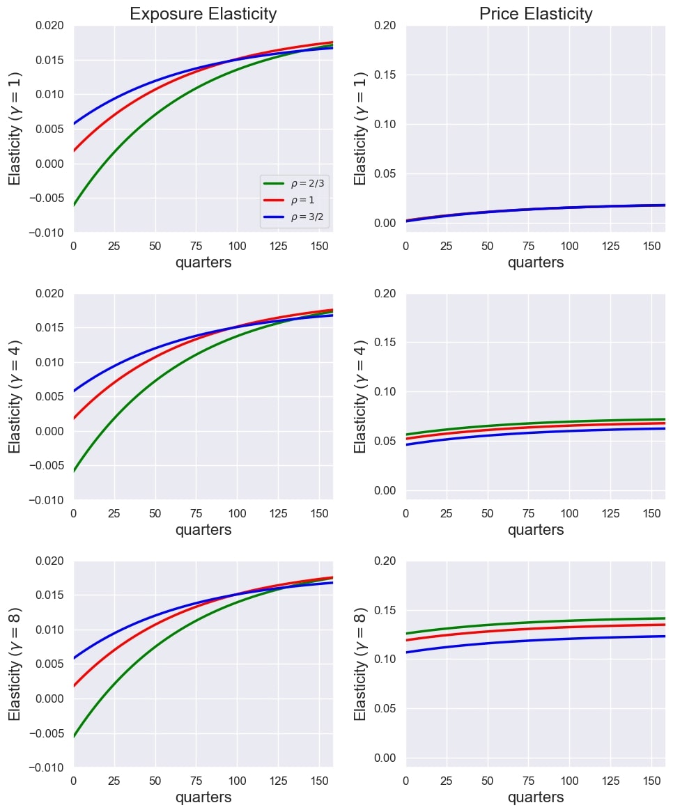
Fig. 11.1 Consumption shock-exposure and price elasticities for the growth-rate shock for different values of \(\rho\) and \(\gamma\). The initial stochastic volatility state is set to its median. Each of the row panels reports computations for different values of \(\gamma\).#
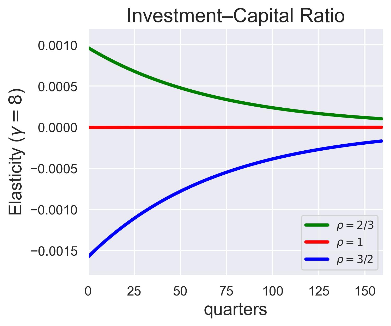
Fig. 11.2 Investment-capital exposure elasticities for the growth rate shock for various values of \(\rho.\) The initial stochastic volatility state is set to its median, and \(\gamma = 8.\)#
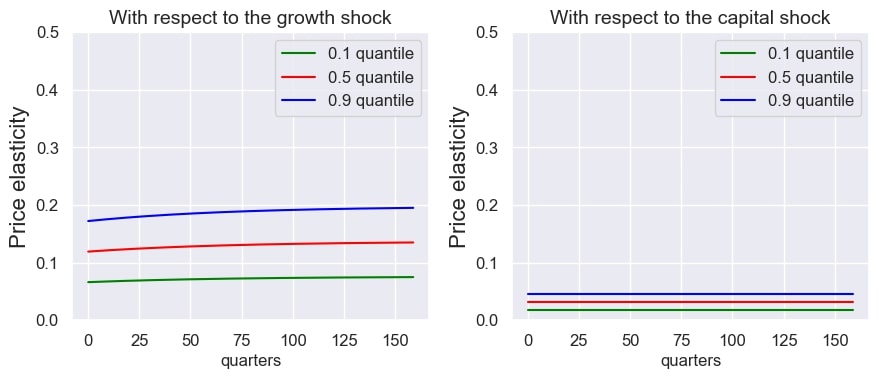
Fig. 11.3 Alternative stochastic volatility quantiles for the price elasticities for the growth and capital shocks. \(\rho = 1, \gamma = 8,\) \(\beta = .99.\)#
Fig. 11.3 gives the shock price elasticities when \(\rho = 1\) and \(\gamma = 8\) for the growth rate shock and the capital shock. Stochastic volatility induces state dependence in these plots as reflected by the quantiles. Since the recursive utility preferences are forward-looking as reflected by the continuation-value contribution to the one-period increment to the stochastic discount factor process (see (11.8)), this forward-looking contribution is reflected in shock price elasticities that are substantially larger for the growth-rate shock.[6] The primary contribution of stochastic volatility is to induce state dependence for the other elasticities as reflected by the quantiles. While the elasticities for the volatility shock are different from zero, their contribution is much smaller than those for the other shocks and thus is not reported in Fig. 11.3.
11.7.5. Another model of intertemporal substitution and complementarity#
We now extend the preference specification of the consumers in the AK model to explore implications of time nonseparability in preferences. We are motivated to do so by rather substantial previous literature. An important earlier contribution is [Ryder and Heal, 1973], which solved a social planner’s problem with stochastic growth. [Sundaresan, 1989], [Constantinides, 1990], [Heaton, 1995], and [Hansen et al., 1999] consider asset pricing implications with internal habit persistence. These papers essentially explore decentralizations of the planner’s problem. The latter paper considers simultaneously a recursive robustness specification as we will do here, although for a different model specification.
[Pollak, 1970] introduced a version of external habit persistence in the consumer demand function. The stock \(H_t\) enters preferences as a societal or external input and not recognizable as an individual input in the current time period. Thus there is an externality induced by this specification of preferences. [Abel, 1990] and [Campbell and Cochrane, 1999] explore implications of external habit persistence, along with many subsequent papers on asset pricing with external habit persistence. Much of the latter literature abstracts from production, but there are exceptions. See for instance, [Lettau and Uhlig, 2000]. The equilibrium solution with external habit persistence deviates from the planner problem because the investor is assumed not to internalize the consumption impact on habits. A benevolent planner would internalize the consumption impact on habits, so the equilibrium with the external habit specification is not socially optimal, opening the door to prudent policy interventions. In what follows we will compare the external and internal habit specifications, where we have dual interpretations of the internal habit version. Either the habits are internalized by the individual decision makers or it provides the socially efficient outcomes for an external habit specification. In the latter case, a prudent policy maker would aim to address these externalities.
Relative to our previous computations, we introduce an additional state variable, which we will call the habit stock, \(H_t\). This stock evolves as:
where \(\nu_h > 0\) is a depreciation rate. This new investment \(I_{h,t}\) is measured consumption. Notice that the coefficients on the right side of the evolution equation sum to one. This allows us to interpret \(H_{t+1}\) as an exponentially weighted arithmetic average of current and past values of measured consumption.
We write the evolution equation in logarithms as
For numerical purposes, we transform this equation to be:
where we treat \(\log H_{t} - \log K_t\) as one of the components of \(X_t\) and we substitute the evolution of \(\log K_{t+1}\) to depict the evolution of this component. As previously, \({\widehat G}_t = \log K_t\).
We modify the output constraint to be:
where \(I_{k,t}\) is the investment in the capital stock. Analogous to the previous formulation, we transform this equation to be:
where \(\frac {I_{h,t}}{K_t} \) and \(\frac {I_{k,t}}{K_t}\) are the two components of \(D_t\).
What enters the utility function each date inside the recursive utility preference specification is the CES aggregate:
for \(\tau \ge 0\). Here and for the remainder of this section, \(\lambda\) denotes the weight in this CES aggregator and not the discounted weight \(\beta \exp\left[(1-\rho) \eta_c^0\right]\) of (11.17) that appears in the approximation formulas. This specification captures a form of intertemporal complementarity and intertemporal substitution in preferences. In static demand theory, \(\tau = 0\) implies perfect substitutes, and when \(\tau > 1\), the preferences display a form of complementarity as reflected in the cross price effects on demand. There is a different notion of intertemporal complementarity as originally defined by [Ryder and Heal, 1973]. Under this notion, increasing \(H_t\), keeping \(I_{h,t}\) fixed should decrease \(C_t\). (They impose other restrictions.) This form of intertemporal complementarity can instead be captured by letting \(\lambda < 0\). Effectively, \(H_t\) is a “bad’’ not a “good,’’ in the CES aggregator. Setting \(0 < \lambda \le 1\) captures a form of consumption durability.
For computational purposes, we divide both sides of (11.38) by \(K_t\) and take logarithms:
Consistent with the habit-persistence literature, we allow the parameter \(\lambda\) to be negative. When \(\tau\) is one, this becomes a Cobb-Douglas specification:
Remark 11.9
The asset pricing literature often features the computationally more challenging case in which \(\tau = 0\) and \(\lambda < 0\). The local approximation methods we describe here could provide a particularly poor approximation for this limiting parameter configuration. In what follows, we will entertain positive values of \(\tau\) that are less than one.
For simplicity, consider the case in which \(\rho = 1\). Recall that \(\rho\) also impacts intertemporal substitution in preferences so by setting it to one we feature the novel contribution coming from this dynamic specification of preferences. While we investigate other specifications of \(\tau\), for the moment suppose that \(\tau = 1\). The first-order conditions for \(D_t \) are:
From the first-order conditions for \(D_{1,t}\), we find that
This depicts the marginal value of \(MS_t\) in terms of both a current marginal utility contribution and a forward-looking piece coming from the planner internalizing the intertemporal contribution to preferences. When this contribution is not internalized, the expectation term is omitted from the first-order conditions.
We choose to use \(I_{h,t}\) as the date \(t\) numeraire instead of \(C_t\), as the former is measured consumption. In light of this choice, the logarithm of the one-period stochastic discount factor is
In our calculations, we approximate \(\log MS_t\) since it enters this formula for the logarithmic stochastic discount factor construction.
In the figures that follow we compare results for the internal specification versus the external specification of preferences, which differ in terms of how the investor views the intertemporal contribution to preferences. There are two ways to interpret these comparisons. One way is as a comparison of two specifications of investor preferences. The other is to presume that the intertemporal contribution to preferences is external from the standpoint of the investor, but what is referred to as internal is a planner solution that internalizes the externality via a policy intervention. Fig. 11.4 gives the shock exposure elasticity for the internal specification and Fig. 11.5 the same for the external specification for a growth-rate shock to the investment-capital ratio. In all cases, \(\rho = 1\) in order to feature this alternative intertemporal substitution mechanism. We report results for different values of \(\lambda\) and \(\tau\). We see in Fig. 11.4 that responses have different signs depending on whether \(\lambda\) is positive or negative. The most pronounced responses are for \(\tau = .01\) for which the two different values of \(\lambda\) have offsetting effects that are roughly comparable. In contrast, for the external specification, the \(\lambda = -2\) responses are in sharp contrast to those of \(\lambda = .67\). The implied intertemporal complementarity in preferences, or so called “habit persistence”, is particularly prominent when \(\tau << 1.\)
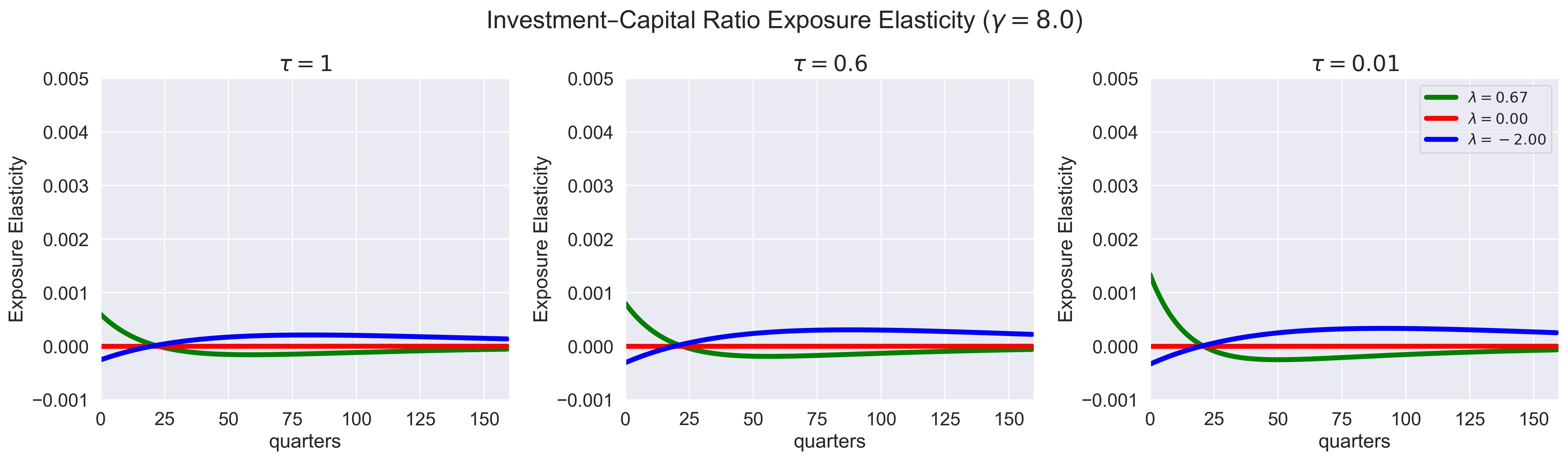
Fig. 11.4 Exposure elasticity of the growth shock in the internal intertemporal preference model for \(\lambda = .67, 0, -2\), \(\gamma = 8\) and different values of \(\tau.\)#
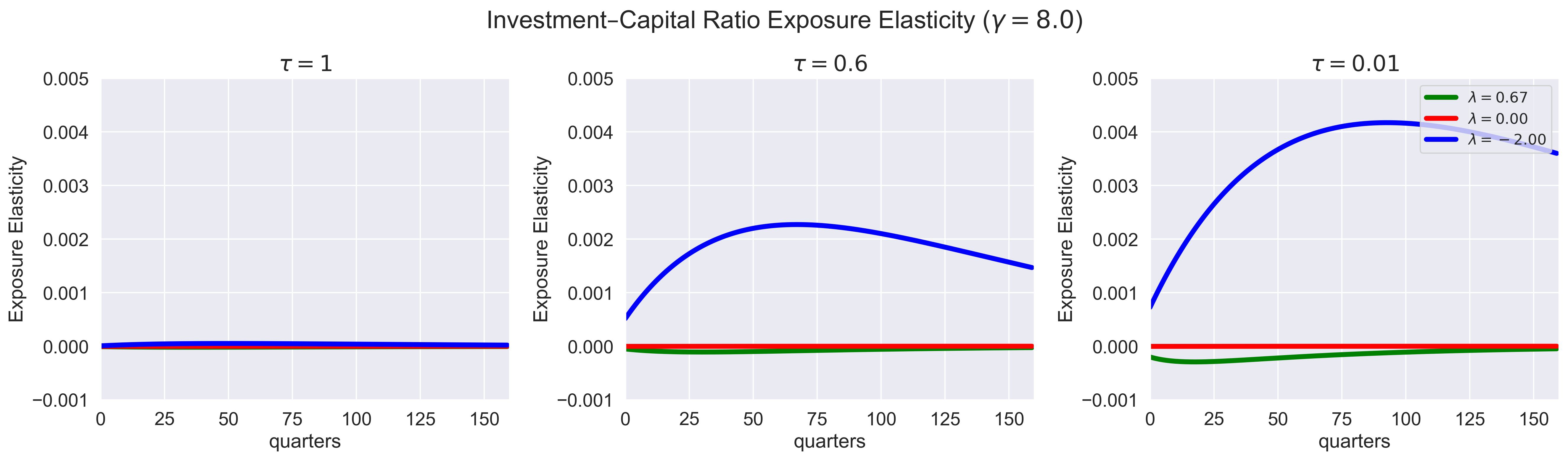
Fig. 11.5 Exposure elasticity of the growth shock in external intertemporal preference model for \(\lambda = .67, 0 , -2\), \(\gamma = 8\) and different values of \(\tau.\)#
Fig. 11.6 and Fig. 11.7 depict the consumption price elasticities for the growth rate shock for both the internal and external specifications when \(\gamma = 8\). We again consider intertemporal substitution (\(\lambda = .67\)) and intertemporal complementarity (\(\lambda = - 2\)). For the internal preference specification the price elasticities are a little bit higher under intertemporal complementarity, but the impact is much more substantial for the external preference specification, particularly when \(\tau=.01\).
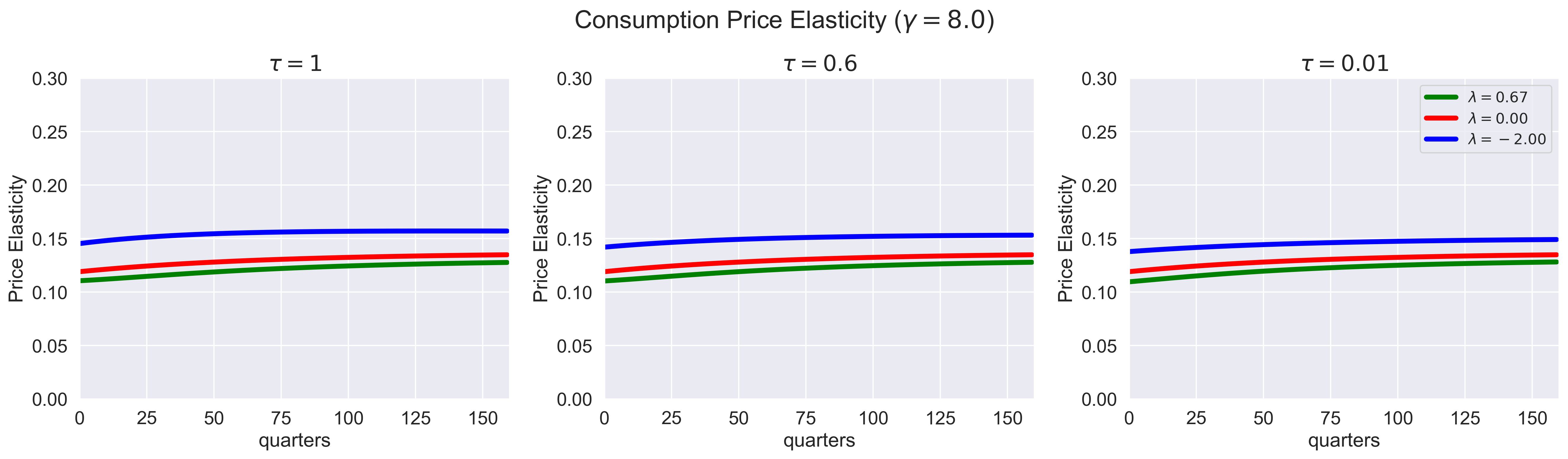
Fig. 11.6 Consumption price elasticity of the growth shock in internal intertemporal preference model for \(\lambda = .67, 0 , -2\), \(\gamma = 8\) and different values of \(\tau.\)#
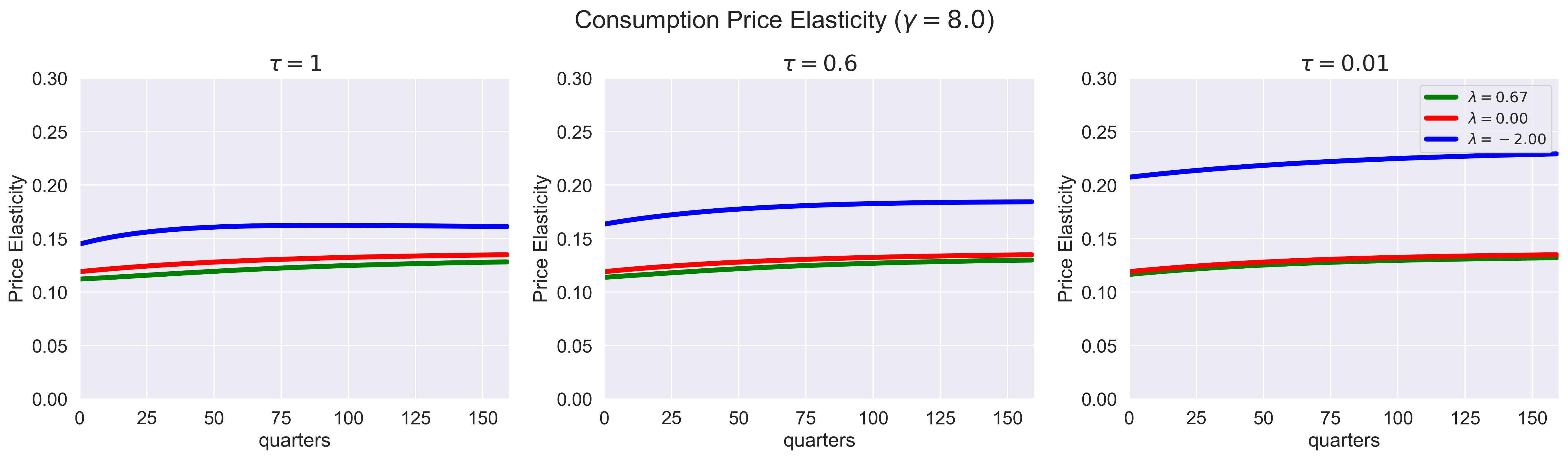
Fig. 11.7 Consumption price elasticity of the growth shock in external intertemporal preference model for \(\lambda = .67, 0 , -2\), \(\gamma = 8\) and different values of \(\tau.\)#
Fig. 11.8 and Fig. 11.9 repeat the plots, except with \(\gamma\) lowered to 4. Perhaps not surprisingly, the price elasticities are now half or less what they were when \(\gamma=8\), but the overall patterns remain the same.
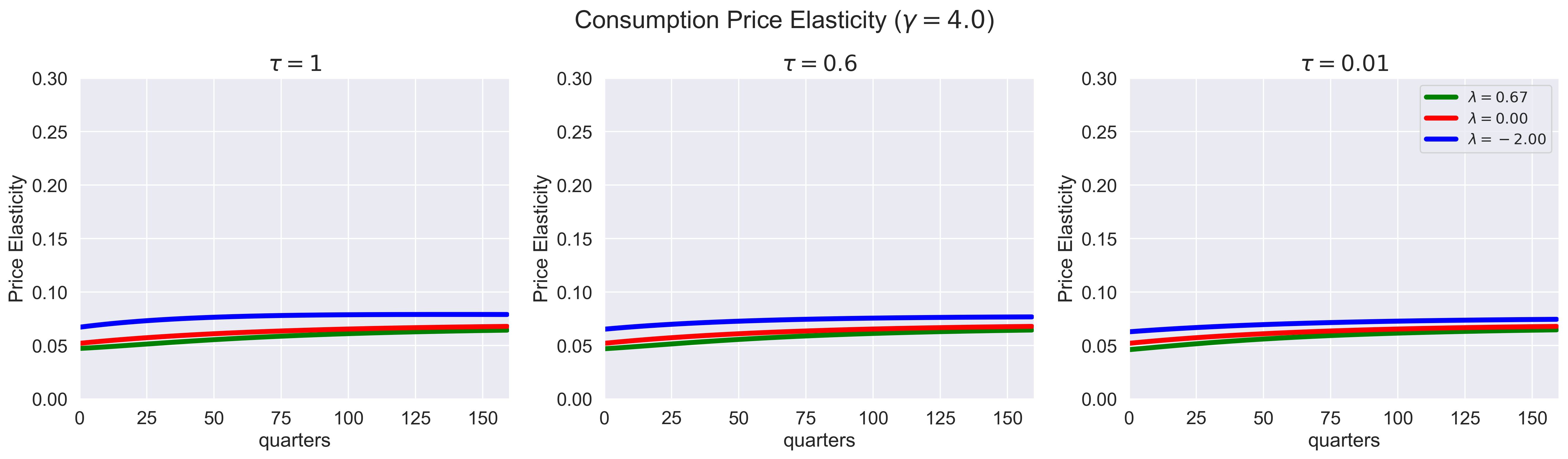
Fig. 11.8 Consumption price elasticity of the growth shock in internal intertemporal preference model for \(\lambda = .67, 0 , -2\), \(\gamma = 4\) and different values of \(\tau.\)#
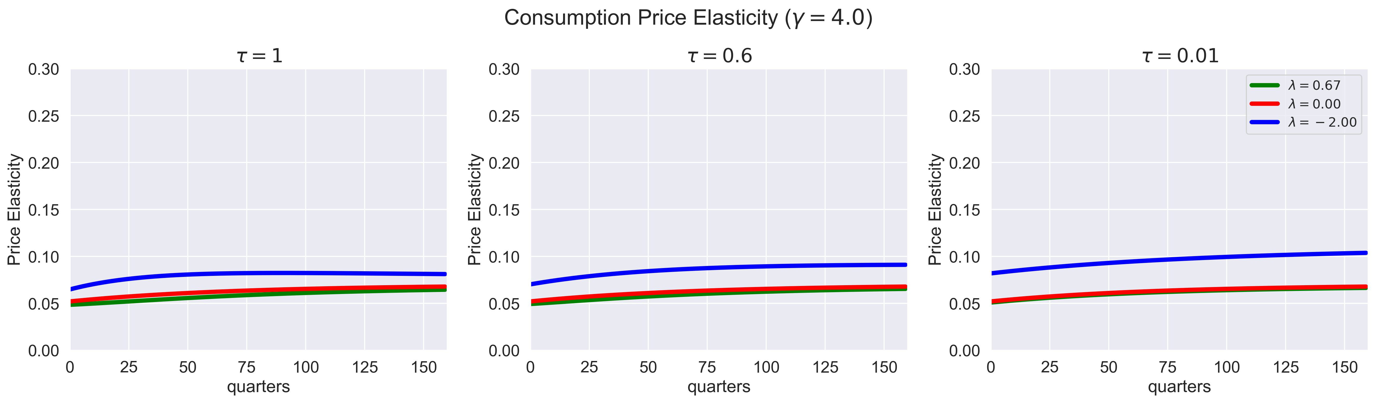
Fig. 11.9 Consumption price elasticity of the growth shock in external intertemporal preference model for \(\lambda = .67, 0 , -2\), \(\gamma = 4\) and different values of \(\tau.\)#
11.8. Solving models#
In this section, we briefly describe one way to extend the approach that builds directly on previous second-order approaches of [Kim et al., 2008], [Schmitt-Grohé and Uribe, 2004], and [Lombardo and Uhlig, 2018]. While such methods should not be viewed as being generically applicable to nonlinear stochastic equilibrium models, they are useful pedagogically and often as initial steps to understanding models that are “smooth.” See [Pohl et al., 2018] for a careful study of nonlinearity in asset pricing models with recursive utility.[7]
We implement these methods for second-order approximation using the following steps.
Solve for the \({\sf q}=0\) deterministic model.
Take as given first and second-order approximate solutions for \({\widehat C}_t - {\widehat G}_t\) and \({\widehat G}_{t+1} - {\widehat G}_t\). Solve for the approximate solutions for \({\widehat V}_t - {\widehat G}_t,\) \({\widehat V}_{t+1} - {\widehat R}_t\) and \(N_{t+1}.\)
Compute the first-order expansion and solve the resulting equations following the previous literature for \(D_t,\) \({\widehat C}_t - {\widehat G}_t,\) and \({\widehat G}_{t+1} - {\widehat G}_t.\) When constructing these equations, use expectations computed using the probabilities induced by \(N_{t+1}^0\). Substitute the first-order approximation for \({\widehat R}_t - {\widehat G}_t.\)
Compute the second-order expansion and solve the resulting equations following the previous literature. Again use the expectations induced by \(N_{t+1}^0\). In addition, make another recursive utility adjustment expressed in terms of the approximations of \({\widehat R}_t - {\widehat G}_t.\)
Return to step 2, and repeat until convergence.
Initialize this algorithm by solving the case \(\gamma_o=1\) and \(\rho = 1,\) which can be computed without iteration.
See the Appendices that follow for more details and formulas to use in the solution method.
As a second approach, we iterate over the approximation to \(N_{t+1}^*\) given by formula (11.30), restricted to induce an alternative probability distribution. Call the approximation \({\widetilde N}_{t+1}\) with an induced distribution for \(W_{t+1}\) that is normal with conditional mean \({\tilde \mu}_t\) and covariance matrix \({\widetilde \Sigma}\).
While we discussed the approximation for resource allocation problems with recursive utility, there is a direct extension of this approach to solve a general class of stochastic equilibrium models by stacking a system of expectational-type equations expressed in part using the recursive utility stochastic discount factor that we derived. For resource allocation problems, we expressed the first-order conditions for the planner in utility units, which simplified some formulas. Equilibrium models not derived from a planner’s problem typically use stochastic discount factors expressed in consumption units when representing investment choices. The approximation methods described in this chapter have a direct extension to such models.
11.9. Summary#
Recursive utility separates risk aversion from intertemporal substitution by replacing the conditional expectation of a continuation value with a risk-adjusted certainty equivalent. The same recursion admits a second reading, as a decision maker who distrusts the model and evaluates plans under a worst case penalized by relative entropy, which is the link back to Chapter 10. Both readings deliver a stochastic discount factor of the form first derived in Section Shadow values of Chapter 4, and they are observationally equivalent within a model even though they differ in interpretation.
Two approximations are developed: a continuous-time limit with Brownian information, and a small-noise expansion modified so that macroeconomic uncertainty has first-order rather than higher-order consequences. These expansions are local in the same sense as the stochastic responses of Chapter 5, and their implications are read off using the shock elasticities of Chapter 9. Chapter 12 applies the apparatus to marginal valuation.
11.10. Exercises#
Exercise 11.1 (The stochastic discount factor by the chain rule)
Remark 11.3 sketches a verification of the one-period stochastic discount factor (11.8) by assembling four marginal utilities. Carry it out.
(a) From the recursions (11.3) and (11.4), compute the four derivatives
(b) Assemble the intertemporal marginal rate of substitution \(\frac{(m{\hat r})(m{\hat v}^+)(mc^+)}{mc}\) and confirm that it reproduces the first line of (11.8).
(c) Show that the two exponential factors combine into \(\beta N_{t+1}^*\exp\left({\widehat S}_{t+1}-{\widehat S}_t\right)\) with \({\widehat S}_{t+1}-{\widehat S}_t\) as in (11.9), and confirm that \(N_{t+1}^*\) has conditional expectation one.
(d) The chapter describes three contributions: a subjective discount factor, a change of measure, and an adjustment for intertemporal substitution. Say which of the three survives when \(\gamma = 1\), and separately when \(\rho = 1\). Which of the two restrictions eliminates the forward-looking element of the one-period discount factor?
Exercise 11.2 (The order-zero approximation and a restriction on discounting)
The order-zero expansion delivers (11.15) for \(\eta_{v-c}^0\), and the order-one weight is \(\lambda = \beta\exp\left[(1-\rho)\eta_c^0\right]\).
(a) Derive (11.15) by imposing the guess \({\widehat V}_t^0 - {\widehat C}_t^0 = \eta_{v-c}^0\) on the order-zero recursion, and solve for \(\eta_{v-c}^0\) explicitly as in (11.16).
(b) Take the limit \(\rho \rightarrow 1\) and verify that \(\eta_{v-c}^0 = \frac{\beta}{1-\beta}\eta_c^0\). Interpret.
(c) Show that requiring \(\lambda < 1\) is equivalent to \((1-\rho)\eta_c^0 < -\log\beta\). Explain why this is a joint restriction on the subjective discount rate and the growth rate rather than on \(\beta\) alone, and describe how it differs according to whether \(\rho < 1\) or \(\rho \ge 1\).
(d) Verify that \(\eta_{v-c}^0\) does not depend on \(\gamma\) or \(\xi\). Why should the order-zero term be free of the uncertainty-aversion parameters, given the expansion protocol (11.11) and the scaling in Section Recursive utility valuation process?
Exercise 11.3 (Order-one continuation values for a scalar autoregression)
Specialize the order-one system (11.24) to a scalar state. Let
with \(|{\sf a}| < 1\), so that \(\psi_{x'} = {\sf a}\), \(\psi_{w'} = {\sf b}\), \(\psi_{\sf q} = 0\), \(\kappa_x = {\sf d}\), \(\kappa_{w'} = {\sf f}\).
(a) Solve (11.24) for \(\upsilon_1\) and \(\upsilon_0\) in closed form.
(b) Verify that \(\upsilon_1\) does not involve \(\gamma_o\) while \(\upsilon_0\) does, and identify the uncertainty-adjustment term in \(\upsilon_0\). What is its sign for \(\gamma_o > 1\)?
(c) Take \(\lambda \rightarrow 1\). Show that \(\upsilon_1 {\sf b} + {\sf f}\) converges to \({\sf f} + \frac{{\sf d}{\sf b}}{1-{\sf a}}\), and identify this object using Chapter 4. Relate your answer to Remark 11.6.
(d) Remark 11.8 reports that under the change of measure induced by \(N_{t+1}^0\) the shock acquires mean \(\mu^0 = -\frac{1}{\xi_o}\left(\upsilon_1\psi_{w'}+\kappa_{w'}\right)'\). Compute it for this scalar case and explain, using (c), the sense in which investors’ concern about long-horizon uncertainty is priced into a one-period valuation.
Exercise 11.4 (Robustness and risk aversion in continuous time)
Section Recursive utility valuation process and the continuous-time limit that follows it establish an equivalence between a risk-adjusted recursion and a penalized minimization. Verify it and then apply it.
(a) Starting from (11.10) with \(\gamma = 1\), introduce the drift distortion \(H_t\) and the entropy penalty \(\frac{\xi}{2}\left|H_t\right|^2\). Solve the minimization for \(H_t^*\).
(b) Substitute \(H_t^*\) back and show that the resulting equation coincides with (11.10) provided that \(\gamma - 1 = 1/\xi\).
(c) [Duffie and Epstein, 1992] call \(\gamma\) a variance multiplier. Using (b), give the robustness reading of that name, and say what \(-H_t^*\) measures in the language of Section Recursive utility valuation process‘s discussion of uncertainty pricing.
(d) Now apply the machinery to the AK economy of Section An economy with long-run uncertainty with \(\rho = 1\). Show that the first-order conditions (11.37) imply that both components of \(D_t\) are constant, solve for \(D_{2,t}^*\), and explain why \({\widehat R}_t - {\widehat G}_t\) drops out. What does this tell you about where \(\gamma\) can and cannot show up in the quantity dynamics, and is that consistent with the elasticity plots Fig. 11.1 and Fig. 11.2?
11.11. Answers#
Solution to Exercise 11.1 (The stochastic discount factor by the chain rule)
(a) Differentiating the homogeneous-of-degree-one recursion (11.1) written in logarithms, or equivalently reading off Remark 11.3,
The third follows from differentiating the certainty equivalent (11.4): the derivative of \(\frac{1}{1-\gamma}\log{\mathbb E}\exp\left[(1-\gamma){\widehat V}_{t+1}\right]\) with respect to \({\widehat V}_{t+1}\) is the exponentially tilted weight.
(b) Multiplying and cancelling the common factor \((1-\beta)\) and the \(\exp\left[(\rho-1)\right]\) terms,
where the \(\exp\left[(1-\rho)({\hat r}-{\hat v})\right]\) from \(m{\hat r}\) and the \(\exp\left[(\rho-1){\hat v}\right]\) from \(mc\) combine with the \(\exp\left[(\rho-1){\hat v}^+\right]\) from \(mc^+\) to leave \(\exp\left[(\rho-1)\left({\hat v}^+-{\hat r}\right)\right]\). Setting \({\hat v}^+ = {\widehat V}_{t+1}\), \(c^+ = C_{t+1}\), \(c = C_t\), \({\hat r} = {\widehat R}_t\) gives the first line of (11.8).
(c) Group the exponentials. The factor \(\exp\left[(1-\gamma)\left({\widehat V}_{t+1}-{\widehat R}_t\right)\right]\) is exactly \(N_{t+1}^*\), by the identity following (11.6). The remaining factor is
which is \(\exp\left({\widehat S}_{t+1}-{\widehat S}_t\right)\) by (11.9). For the conditional expectation,
by the definition (11.4) of \({\widehat R}_t\).
(d) All three factors are present in general. Setting \(\gamma = 1\) makes \(N_{t+1}^* \equiv 1\): the change of measure disappears, and the discount factor reduces to \(\beta\exp\left({\widehat S}_{t+1}-{\widehat S}_t\right)\) with \(\rho\) still shaping intertemporal substitution. Setting \(\rho = 1\) makes \({\widehat S}_{t+1}-{\widehat S}_t = -\left({\widehat C}_{t+1}-{\widehat C}_t\right)\), the logarithmic-utility term, while \(N_{t+1}^*\) survives.
It is \(\gamma = 1\) that removes the forward-looking element. The continuation value \({\widehat V}_{t+1}\) enters the one-period discount factor only through \(N_{t+1}^*\); when \(\gamma = 1\) that channel closes and the discount factor depends on nothing beyond date \(t+1\) consumption. This is the observation the chapter makes when it says that the risk contribution “introduces a long-term impact on short-term valuation,” and it is the mechanism that Exercise 11.3 quantifies.
Solution to Exercise 11.2 (The order-zero approximation and a restriction on discounting)
(a) At order zero randomness vanishes, so \({\widehat R}_t^0 = {\widehat V}_{t+1}^0\). Substituting the guess into the order-zero counterpart of (11.3) and using \({\widehat C}_{t+1}^0 - {\widehat C}_t^0 = \eta_c^0\),
Collecting the terms in \(\exp\left[(1-\rho)\eta_{v-c}^0\right]\) gives (11.15), and taking logarithms gives (11.16):
(b) As \(\rho \rightarrow 1\) both numerator and denominator vanish. Expanding \(\exp\left[(1-\rho)\eta_c^0\right] \approx 1 + (1-\rho)\eta_c^0\), the numerator becomes \(-\log\left(1-\beta-\beta(1-\rho)\eta_c^0\right) + \log(1-\beta) \approx \frac{\beta(1-\rho)\eta_c^0}{1-\beta}\), so
With logarithmic period utility the continuation value is the discounted sum of expected future log consumption. \(\frac{\beta}{1-\beta}\) counts future periods, each growing by \(\eta_c^0\).
(c) From the derivation of \(\lambda\) in Section Recursive utility valuation process, \(\lambda = \beta\exp\left[(1-\rho)\eta_c^0\right]\), so \(\lambda < 1\) is \(\log\beta + (1-\rho)\eta_c^0 < 0\), that is \((1-\rho)\eta_c^0 < -\log\beta\).
This restricts the subjective discount rate \(-\log\beta\) relative to the growth rate \(\eta_c^0\), not \(\beta\) in isolation, because the effective rate at which the future is discounted in the transformed problem nets out growth. When \(\rho < 1\) the left side is positive for a growing economy, so the subjective discount rate must exceed a strictly positive lower bound: a patient enough agent facing a growing endowment has an unbounded objective. When \(\rho \ge 1\) the left side is nonpositive and the restriction is slack for any \(\beta < 1\); growth then reduces rather than raises the effective discount rate, because with an intertemporal elasticity of substitution below one the agent dislikes postponing consumption enough to offset its growth.
(d) Inspection of (11.16) shows only \(\beta\), \(\rho\), and \(\eta_c^0\). The perturbation parameter \({\sf q}\) multiplies the shocks in (11.11), and the order-zero term is the \({\sf q} = 0\) limit, in which all randomness has been switched off. Uncertainty aversion is aversion to randomness, so with nothing to be averse to it can play no role.
The chapter’s device of letting \(\gamma - 1 = (\gamma_o-1)/{\sf q}\) prevents this from making uncertainty irrelevant everywhere: aversion grows as the shocks shrink, so that the product survives, and the adjustment reappears at order one in \(\upsilon_0\) rather than being pushed to order two. Section Recursive utility valuation process puts it that “the variable \({\sf q}\) is doing double duty.”
Solution to Exercise 11.3 (Order-one continuation values for a scalar autoregression)
(a) The first equation of (11.24) reads \(\upsilon_1 = \lambda\left({\sf a}\upsilon_1 + {\sf d}\right)\), so
With \(\psi_{\sf q} = 0\), the second equation is \(\upsilon_0 = \lambda\left(\upsilon_0 + \kappa_{\sf q} + \frac{1-\gamma_o}{2}\left(\upsilon_1{\sf b}+{\sf f}\right)^2\right)\), so
(b) \(\upsilon_1\) involves only \(\lambda, {\sf a}, {\sf d}\); the uncertainty-aversion parameter enters nowhere. Its role is confined to the constant, through
which is negative for \(\gamma_o > 1\) and becomes more so as \(\gamma_o\) rises. So greater uncertainty aversion lowers the level of the continuation value without altering how it responds to the state.
(c) As \(\lambda \rightarrow 1\), \(\upsilon_1 \rightarrow \frac{\sf d}{1-{\sf a}}\) and therefore
which is the scalar case of \({\mathbb F} + {\mathbb D}\left({\mathbb I}-{\mathbb A}\right)^{-1}{\mathbb B}\), the coefficient on the martingale increment in (4.6) of Chapter 4. Its square is the variance of the permanent shock to log consumption. This is what Remark 11.6 asserts: the limiting variance converges to the variance of the martingale increment of \({\widehat C}^1\).
(d) Here \(\mu^0 = -\frac{1}{\xi_o}\left(\upsilon_1{\sf b}+{\sf f}\right)\), a scalar. By (c), for \(\lambda\) near one this is \(-\frac{1}{\xi_o}\left({\sf f}+\frac{{\sf d}{\sf b}}{1-{\sf a}}\right)\): the mean of the one-period shock is displaced by an amount proportional to the cumulative response of consumption to that shock.
\(N_{t+1}^*\) prices a shock by how much it moves \({\widehat V}_{t+1}\). \({\widehat V}_{t+1}\) discounts all future consumption growth, so its sensitivity to a shock aggregates the whole impulse response. A shock with a small immediate effect \({\sf f}\) but a persistent one, so that \({\sf d}{\sf b}/(1-{\sf a})\) is large, is heavily priced at a one-period horizon even though almost nothing happens to consumption within that period.
The same \(\mu^0\) arises from an agent who fears that his model of the persistent component is wrong, since \(\gamma_o - 1 = 1/\xi_o\). Remark 11.8 notes that Chapter 6 showed the variance of that object to be poorly estimated. \(\gamma_o\) does double duty as a taste and as a confidence. The data speak weakly to the magnitude it prices.
Solution to Exercise 11.4 (Robustness and risk aversion in continuous time)
(a) With \(\gamma = 1\) and a drift distortion, the recursion becomes
The objective is a strictly convex quadratic in \(H_t\); its first-order condition is \(\sigma_t^V + \xi H_t = 0\), so
(b) Substituting back, \(\sigma_t^V\cdot H_t^* + \frac{\xi}{2}\left|H_t^*\right|^2 = -\frac{1}{\xi}\left|\sigma_t^V\right|^2 + \frac{1}{2\xi}\left|\sigma_t^V\right|^2 = -\frac{1}{2\xi}\left|\sigma_t^V\right|^2\), so the minimized equation is
Comparing with (11.10), whose corresponding term is \(\frac{1-\gamma}{2}\left|\sigma_t^V\right|^2\), the two agree exactly when \(\frac{1-\gamma}{2} = -\frac{1}{2\xi}\), that is \(\gamma - 1 = 1/\xi\).
(c) (11.10) shows the continuation value’s local mean penalized by \(\frac{\gamma}{2}\left|\sigma_t^V\right|^2\), so larger \(\gamma\) multiplies the local variance more heavily, which is the sense in which it is a variance multiplier. Part (b) says that the same multiplier is what an agent would apply if, instead of being risk averse, he were confident only to within an entropy budget of size \(1/\xi = \gamma - 1\) and evaluated plans at the worst drift within that budget. A large variance multiplier and a small entropy penalty are the same equation.
The vector \(-H_t^* = \frac{1}{\xi}\sigma_t^V\) is the vector of local uncertainty prices: the compensation, expressed as a shift in a conditional mean, required for bearing exposure to each Brownian increment. Compounding these into the exponential martingale \(M_t^*\) produces the change of measure under which asset prices are computed.
(d) With \(\rho = 1\) the exponential factors in (11.37) are all unity, so the two first-order conditions become
Neither involves \({\widehat R}_t - {\widehat G}_t\), which is the only place the continuation value could have entered: at \(\rho = 1\) the exponent \((1-\rho)\) annihilates it. Combining the two with the resource constraint \(D_{1,t} = \alpha - D_{2,t}\) and solving,
a constant, independent of the state and independent of \(\gamma\).
So at \(\rho = 1\) the parameter \(\gamma\) cannot affect the quantity allocation at all; investment and consumption ratios are pinned down by \(\beta\), \(\alpha\), and the adjustment-cost parameter \(\zeta\) alone. It can and does affect prices, through \(N_{t+1}^*\) in the stochastic discount factor.
The figures show this pattern. Fig. 11.2 shows the investment-capital exposure elasticities responding sharply to \(\rho\), with the sign of the initial response flipping around \(\rho = 1\), while the accompanying discussion reports that \(\gamma\) has “virtually no impact on the quantity elasticities” and a large impact on the price elasticities. The algebra here explains why: at \(\rho = 1\) the separation is exact, and away from \(\rho = 1\) it is broken only through the \({\widehat R}_t - {\widehat G}_t\) term, which is a second-order channel.