
10. Risk, Ambiguity, and Misspecification[1]#
Authors: Lars Peter Hansen (University of Chicago) and Thomas Sargent (NYU)
\(\newcommand{\eqdef}{\stackrel{\text{def}}{=}}\)

Pioneers in Uncertainty and Decision Theory. Frank Knight, Abraham Wald, and Jimmie Savage.
“Uncertainty must be taken in a sense radically distinct from the familiar notion of risk, from which it has never been properly separated…. and there are far-reaching and crucial differences in the bearings of the phenomena depending on which of the two is really present and operating.” [Knight, 1921]
“The only uncertainty we can rely on is blind chance.” Attributed to Ludvig Beethoven during Napoleonic Wars.
10.1. Introduction#
We refer to a likelihood function as a parameterized probability distribution, while a prior probability distribution describes a decision maker’s subjective beliefs about those parameters.[2] This chapter brings recent contributions to decision theory into contact with statistics and econometrics by distinguishing roles played by likelihood functions and prior probability distributions. We do this to address some practical econometric concerns about misspecifications of the parameterized probability distributions themselves, as well as doubts about appropriate prior probabilities.
To address these concerns, we combine ideas from control theories — which construct decision rules that are robust to a class of model misspecifications — with axiomatic decision theories created by economic theorists. Such decision theories originated with axiomatic formulations by von Neumann and Morgenstern, Savage, and Wald ([Wald, 1947, Wald, 1949, Wald, 1950], [Savage, 1954]). Ellsberg ([Ellsberg, 1961]) pointed out that Savage’s framework seems to include nothing that could be called “uncertainty” as distinct from “risk”. Theorists after Ellsberg constructed coherent systems of axioms that embrace a notion of ambiguity aversion. Remarkably from our point of view, most such axiomatic formulations of decision making under uncertainty in economics are not cast explicitly in terms of likelihood functions and prior distributions over parameters.
We want to reinterpret objects that appear in some of those axiomatic foundations of decision theories in ways useful to an econometrician. We use an axiomatic structure to express ambiguity about a prior over a family of statistical models, on the one hand, along with concerns about misspecifications of those models, on the other hand.
More specifically, we align definitions of statistical models, uncertainty, and ambiguity with ideas from decision theories that build on [Anscombe and Aumann, 1963]’s way of representing subjective and objective uncertainties. We connect our analysis to econometrics and robust control theory by using Anscombe-Aumann states as parameters that index alternative statistical models of random variables affecting outcomes that a decision maker cares about. By modifying aspects of [Gilboa et al., 2010], [Cerreia-Vioglio et al., 2013], and [Denti and Pomatto, 2022], we show how to use variational preferences to represent uncertainty about priors and also concerns about statistical model misspecifications.
Although they proceeded differently than we do here, [Chamberlain, 2020], [Cerreia-Vioglio et al., 2013], and [Denti and Pomatto, 2022] studied related issues. [Chamberlain, 2020] emphasized that likelihoods and priors are both vulnerable to potential misspecifications. He focused on uncertainty about predictive distributions constructed by integrating likelihoods with respect to priors. In contrast to Chamberlain, we formulate a decision theory that distinguishes uncertainties about priors from uncertainties about likelihoods. [Cerreia-Vioglio et al., 2013] (section 4.2) provided a rationalization of the smooth ambiguity preferences proposed by [Klibanoff et al., 2005] that includes likelihoods and priors as components. [Denti and Pomatto, 2022] extended this approach by using an axiomatic revealed preference method to deduce a parameterization of a likelihood function. However, neither [Cerreia-Vioglio et al., 2013] nor [Denti and Pomatto, 2022] sharply distinguished prior uncertainty from concerns about misspecifications of likelihood functions. We want to do that. We formulate concerns about statistical model misspecifications as uncertainty about likelihoods.
Discrepancies between two probability distributions occur throughout our analysis. They help us to connect our framework to some models in “behavioral” economics and finance. The decision makers inside some of those models have expected utility preferences in which an agent’s subjective probability – typically a predictive density – differs systematically from the predictive density that the model builder assumed governs the data.[3] Other “behavioral” models focus on putative differences among agents’ degrees of confidence in their views of the world. Our framework implies that the form taken by a “lack of confidence” ought to depend on the probabilistic concept about which a decision maker is uncertain, in particular, either a likelihood or a prior or a predictive distribution. Preference structures that we describe in this chapter allow us to formalize different amounts of “confidence” about details in the specification of particular statistical models, on one hand, and about subjective probabilities to attach to alternative statistical models, on the other hand. Our representations of preferences provide ways to characterize degrees of confidence in terms of statistical discrepancies between alternative probability distributions.[4]
10.2. Background motivation#
We are sometimes told that we live in a “data rich” environment. Nevertheless, data are often not “rich” along all of the dimensions that we care about for decision making. Furthermore, data don’t “speak for themselves”. We have to make them speak by positing a family of statistical models indexed by parameters that the data can help us infer. For instance, see [Hansen, 2019] for an elaboration. Thus, despite the ‘’data rich’’ hype, the type of learning we actually do is to infer parameters of a family of statistical models.
Doubts about what existing evidence has taught us about some important dimensions have led some scientists to think about what they call “deep uncertainties.” For example, in a recent paper we read:
“The economic consequences of many of the complex risks associated with climate change cannot, however, currently be quantified. … these unquantified, poorly understood and often deeply uncertain risks can and should be included in economic evaluations and decision-making processes.” [Rising et al., 2022]
In this chapter, we formulate “deep uncertainties” as a lack of confidence in how we represent probabilities of events and outcomes that are pertinent for designing tax, benefit, and regulatory policies. We do this by confessing ambiguities about probabilities, though necessarily in a restrained way.
In our experience as macroeconomists, model uncertainties are not taken seriously enough, too often being dismissed as being of “second-order”, whatever that means in various contexts. In policy-making settings, there is sometimes a misplaced wisdom that acknowledging uncertainty should tilt decisions toward passivity. But in other times and places, one senses that model uncertainty emboldens pretense. As Hayek warned:
“Even if true scientists should recognize the limits of studying human behavior, as long as the public has expectations, there will be people who pretend or believe that they can do more to meet popular demand than what is really in their power.” [Hayek, 1989]
As economists, part of our job is to delineate tradeoffs. Explicit incorporation of precise notions of uncertainty allows us to explore two tradeoffs pertinent to decision making. The first tradeoff concerns how to weigh alternative models. Difficult tradeoffs emerge when we consider implications from multiple statistical models and alternative parameter configurations. Thus, when making decisions, how much weight should we assign to best “guesses” in the face of our model specification doubts, versus bad outcomes that our doubts might unleash? Focusing exclusively on best guesses can lead us naively to ignore adverse possibilities worth considering. Focusing exclusively on worrisome bad outcomes can lead to extreme policies that perform poorly in more normal outcomes. Such considerations induce us to formalize tradeoffs in terms of explicit expressions of aversions to uncertainty.
The second tradeoff is intertemporal: should we act now, or should we wait until we have learned more? While waiting is tempting, it can also be so much more costly that it becomes prudent to take at least some actions now even though we anticipate knowing more later.
10.2.1. Aims#
With these tradeoffs in mind, in this chapter we allow for uncertainties that include
risks: unknown outcomes with known probabilities.
ambiguities: unknown weights to assign to alternative probability models.
misspecifications: unknown ways in which a model provides flawed probabilities.
We will focus on formulations that are enlightening as well as tractable.
10.3. Decision theory overview#
Decision theories under uncertainty provide axiomatic formulations of “rationality.” Since there are multiple such formulations of decision making under uncertainty, it is perhaps best to replace the term “rational” with “prudent.” While these axiomatic formulations are of intellectual and substantive interest, in this chapter we will focus on the implied representations. We think that this approach is interesting because we sympathise with Savage’s own perspective on his axiomatic formulation:
“Indeed the axioms have served their only function in justifying the existential parts of Theorems 1 and 3; in further exploitation of the theory, …, the axioms themselves can end, in my experience, and should be forgotten.” [Savage, 1952]
Later in this chapter, for interested readers, we will delineate specific links to axiomatic formulations of [Savage, 1954] along with [Anscombe and Aumann, 1963]. As a bit of intellectual history, [Anscombe and Aumann, 1963] provided a different way to justify Savage’s representation of decision making in the presence of subjective uncertainty. They prominently feature the distinction between a “horse race” and a “roulette wheel”. They rationalize preferences over acts, where an act maps states into lotteries over prizes. The latter is the counterpart to a roulette wheel. Probability assignments over states then become the subjective input and the counterpart to the “horse race.”
[Anscombe and Aumann, 1963] used this formulation to extend the von Neumann-Morgenstern expected utility with known probabilities to decision problems where subjective probabilities also play a central role as in Savage’s approach. While [Anscombe and Aumann, 1963] provides an alternative derivation of subjective expected utility, many subsequent contributions used the Anscombe-Aumann framework to extend the analysis to incorporate forms of ambiguity aversion. Prominent examples include [Gilboa and Schmeidler, 1989] and [Maccheroni et al., 2006]. In what follows, we provide a statistical slant to such analyses.
10.3.1. Approach#
In this chapter we will use representations implied by modifications and extensions of Savage-style axiomatic formulations. The extensions allow us to incorporate notions of uncertainty beyond risk, motivated by [Knight, 1921] and the subsequent literature that we noted. The overall aim is to make contact with applied challenges in economics and other disciplines. We will start with the basics of statistical decision theory and then proceed to explore extensions that distinguish concerns about potential misspecifications of likelihoods from concerns about the misspecification of priors. This opens the door to better ways of conducting uncertainty quantification for stochastic economic models used for private sector planning and governmental policy assessment. Our task in this chapter is to provide tractable and revealing methods for exploring sensitivity to subjective uncertainties, including potential model misspecification and ambiguity across models. This will allow us systematically to:
assess the impact of uncertainty on prudent decision or policy outcomes;
isolate the forms of uncertainty that are most consequential for these outcomes.
To make the methods tractable and revealing, we will utilize tools from probability and statistics to limit the type and amount of uncertainty that is entertained. As inputs, the resulting representations of objectives for decision making will require a specification of aversion to or dislike of uncertainty about probabilities over future events.
10.3.2. Basic setup#
Our analysis uses the following components.
A parameterized family of models: Models are expressed in terms of densities of a random vector with realization \(x\) and indexed by a parameter \(\theta\) with probabilities given by: \( \ell(x \mid \theta) d \tau(x) \) where
\[\int_{\mathcal X} \ell(x \mid \theta) d \tau(x) = 1.\]In this depiction of probability models, \(\theta \in \Theta\) and \(\Theta\) is a parameter space, \(\mathcal X\) is the space of possible realizations of \(x\), and \(d \tau\) is a measure used in conjunction with the model-specific densities. We refer to \(\ell\) as a likelihood and the probability implied by each \(\theta\) as a structured probability model.
A partitioning of \(\mathbf{x = (w, z)}\): The vector \(z,\) consists of observations or signals that are observed when decisions are made, and the vector \(w\) is an outcome or shock that is realized after decisions are made. For instance, in an intertemporal context, \(w\) may reflect future shocks.
A prize rule: Denoted by \(\gamma,\) a prize rule maps \(\mathcal X\) into prizes, which are the argument of a utility function, \(U.\) We allow the utility function to depend on the unknown parameter \(\theta,\) as is common in statistical decision problems. Arguably, such a formulation is a shorthand for a more primitive specification in which the parameter has ramifications for a future prize that is left unmodeled.
A risk function: The risk function is the expected utility for a prize rule as a function conditioned on the parameter vector \(\theta\):[5]
\[{\overline {U}}(\gamma \mid \theta) = \int_{\mathcal X} {U}[\gamma(x), \theta] \ell(x \mid \theta) d \tau(x) .\]This construct was initiated in a foundational paper by [Wald, 1947] and embraced in part expected utility under known probabilities as rationalized previously by [Ramsey, 1931] and [Von Neumann and Morgenstern, 1944].
A decision rule: Denoted by \(\mathbf{\delta},\) A decision rule is a function of the observations or signals. Decision rules are restricted to be in a set \(\Delta.\) Since a decision rule can depend on \(z\) , ex post learning is entertained. A decision rule gives a restriction on a prize rule via a mapping:
A prior distribution, \(\bf{\pi},\) over the parameter space \(\Theta\): We will sometimes have reason to focus on a particular prior, \(\pi\), that we will call a baseline prior. The unique specification of prior from a Bayesian perspective is a subjective input sometimes referred to as “personalized probability.”
Note that preferences over prize rules imply a ranking over decision rules, the \(\delta\)’s, in \(\Delta\). While we feature the impact of a decision rule on a prize rule, we may extend the analysis to allow \(\delta\) to influence \(\ell\) as happens when we entertain experimentation.
10.3.3. Acts#
We now digress a bit and provide a mapping from our formulas into languages used in axiomatic decision theory. A central construct in that literature is an act. We suggest two constructions of acts, we call the first one a Savage act and the second one an Anscombe-Aumann act. While [Savage, 1954] is an earlier formulation of an axiomatic defense for expected utility constructed with subjective probabilities, the subsequent [Anscombe and Aumann, 1963] formulation has been featured in a variety of extensions of expected utility.
We connect to [Savage, 1954] by defining a state to be a parameter value \(\theta \in \Theta,\) and a consequence to be a probability measure over \({\mathcal C}.\) A Savage act maps each \(\theta\) into a probability distribution over \({\mathcal C}\). For our analysis, the acts of interest use the probability measure that is induced by prize rule \(\gamma(x)\) in conjunction with \(\ell(x \mid \theta) d\tau(x)\) for each state \(\theta\). We assume a linear utility function over consequences as given by:
for a probability measure \(p\) over \({\mathcal C}.\)
To provide connection to [Anscombe and Aumann, 1963], we let \({\mathcal C}\) be the space of consequences. An Anscombe-Aumann act maps each \(\theta \in \Theta\) into a probability measure over \({\mathcal C}.\). Again we may use a prize rule, \(\gamma(x)\) in conjunction with the parameterized family \(\ell(x \mid \theta) d\tau(x)\) to induce a probability measure over \({\mathcal C}\). The utility function remains the same.
[Anscombe and Aumann, 1963] used a roulette wheel analogy for the outcome of an act, and a horse race analogy for a distribution over \(\Theta\). In our setup, we may think of Wald’s risk function as reflecting a roulette wheel type contribution to expected utility.
10.3.4. A simple application#
As an illustration, we consider a model selection problem. Suppose \(\Theta = \{\theta_1, \theta_2\},\) and that the decision maker can use the entire underlying random vector. Thus, we make no distinction between \(\gamma\) and \(\delta\) and no distinctions between \(x\) and \(z\).
The decision rule, \(\delta = \gamma\) is a mapping from \(\mathcal Z\) to \([0,1]\) where \(\delta(z) = 1\) means that the decision maker selects model \(\theta_1\) and \(\delta(z) = 0\) means that the decision maker selects model \(\theta_2.\) We allow for intermediate values between zero and one, which can be interpreted as randomization. These intermediate choices will end up not being of particular interest for this example.
The utility function for assessing risk is:
where \(\upsilon_1,\) and \(\upsilon_2\) are positive utility parameters.
A class of decision rules, called threshold rules, will be of particular interest. Partition \(\mathcal Z\) into two sets:
where the intersection of \(\mathcal Z_1\) and \(\mathcal Z_2\) is empty. A threshold rule has the form:
For a threshold rule, the risk function (the expected utility conditioned on \(\theta\) is:
Suppose that the utility weights \(\upsilon_1\) and \(\upsilon_2\) are both one. Under this threshold decision rule, \(1 - {\overline {U}}(\gamma \mid \theta_1)\) is the probability of making a mistake when model \(\theta_1\) generates the data, and \(1 - {\overline {U}}(\gamma \mid \theta_2)\) is the probability of making a mistake if model \(\theta_2\) generates the data. In statistics, the first of these is called a Type I error, and the second a Type II error, assuming we consider \(\theta_1\) to be the “null model” and \(\theta_2\) to be the “alternative model.” The utility weights determine the relative importance, to the decision maker, of making a correct identification of the model.
10.4. Subjective expected utility#
Under subjective expected utility, we order preferences over \(\gamma\), and hence \(\delta\), by
for a specific \(\pi.\) This representation is supported by Savage and Anscombe-Aumann axioms, but imposes full confidence with no potential misspecification of the priors or the likelihood.
We use these preferences for a decision problem where prize rules are restricted to be in the set \(\Gamma(\Delta)\):
Problem 11.1
Recall the partitioning of \(x = (w, z)\) where the decision rule can only depend on \(z\) and the prize rule on the entire \(x\) vector. Factor \(\ell(\cdot \mid \theta)\) and \(\tau\) as:
In particular, the density \(\ell_2\) captures the probabilities of the shock after observing data, \(z\). These factorizations allow us to write the objective as:
Notice that even if the utility function \({U}\) does not depend on \(\theta\), this dependence may emerge after we integrate over \({\mathcal W}\) in the innermost integration because of the dependence of \(\ell_2(\cdot \mid \theta)\) on the unknown parameter.
10.4.1. Making a decision#
To solve problem (10.1), it is convenient to exchange the orders of integration in the objective:
The \(\gamma\)’s of interest are those that are built from decision rules, the \(\delta\)’s. As \(\delta\) only depends on \(z\) and the objective is additively separable in \(z\), we may equivalently solve a conditional problem using the objective:
for each value of \(z\) provided that the restrictions imposed on \(\delta\) by the construction of the set of decision rules \(\Delta\) are separable in \(z\). That is, provided that we can write:
for given constraint sets \(\Delta(z),\) we may solve
Problem 11.2
Finally, observe that
is the Bayesian posterior distribution for \(\theta.\) Equivalently, we may solve the conditional Bayesian problem:
Problem 11.3
since in forming the objective of conditional problem, (10.5), we divided the objective for the conditional problem, (10.4) by a function of \(z\) alone.
This outcome justifies a distinct role for a statistician to produce a posterior distribution for the parameter vector based on empirical evidence and a decision-maker that takes this posterior as input and makes decisions.
10.4.2. A simple application reconsidered I#
For illustration purposes, consider the example given in Section A simple application. In this example, \(x = z\) and there is no \(w\) contribution. Impose prior probabilities, \( \pi(\theta_1),\) and \( \pi(\theta_2) = 1 - \pi(\theta_1)\) on the two models. Compute the Bayesian posterior probabilities for each value of \(\theta,\)
Consider the conditional problem. If the decision maker chooses model one, then the conditional expected utility is \( \upsilon_1 \bar \pi (\theta_1 \mid z) \) and similarly for choosing model two. Thus the Bayesian decision maker computes:
and chooses a model in accordance with this maximization. This maximization is equivalent to
expressed in terms of the prior, likelihood, and utility contributions. Taking logarithms and rearranging, we see that model \(\theta_1\) is selected if
If the right side of this inequality is zero, say because prior probabilities are the same across models and utility weights are also the same, then the decision rule says to maximize the log likelihood. More generally, both prior probabilities and utility weights come into play.
Notice that this decision rule is a threshold rule where we use the posterior probabilities to partition the \(\mathcal Z\) space. The subset \(\mathcal Z_1\) contains all \(z\) such that inequality (10.6) is satisfied with a weak inequality. We arbitrarily include the indifference values in \({\mathcal Z}_1\).
The Bayesian solution to the decision problem is posed assuming full confidence in a subjective prior distribution. In many problems, including ones with multiple sources of uncertainty, such confidence may well not be warranted. Such a concern might well have been the motivation behind Savage’s remark:
… if I knew of any good way to make a mathematical model of these phenomena [vagueness and indecision], I would adopt it, but I despair of finding one. One of the consequences of vagueness is that we are able to elicit precise probabilities by self-interrogation in some situations but not in others.
— Personal communication from L. J. Savage to Karl Popper, 1957
10.5. An extreme response#
Having assumed full confidence in a prior, suppose we now go to the other extreme and avoid imposing a prior altogether. Construct preferences by computing the conditional (on \(\theta\)) expected utilities, the risk function, for each \(\theta \in \Theta\). Then \(\gamma_2\) is preferred to \(\gamma_1\) if the conditional expected utility of the former exceeds that of the latter for all \(\theta \in \Theta\). This, however, only implies a partial ordering among prize rules. Many such rules cannot be ranked. This partial ordering gives rise to a construct called admissibility, where an admissible \(\delta \in \Delta\) cannot be dominated in the sense of this partial order.
10.5.1. Constructing admissible decision rules#
One way to construct an admissible decision rule is to impose a prior and solve the resulting Bayesian decision problem. We give two situations in which this result necessarily applies, but there are other settings where this result is known to hold.
Proposition 10.1
If an ex ante Bayesian decision problem, (10.1), has a unique solution, then this Bayesian solution is admissible.
Proof. Let \({\tilde \delta}\) be a decision rule that weakly dominates a Bayesian decision rule, \(\delta\), in the sense that
for all \(\theta \in \Theta.\) The \(\tilde \delta\) must also solve the ex ante Bayesian decision problem. Since the solution to the ex ante decision problem is unique, \({\tilde \delta} = \delta\).
Proposition 10.2
Suppose \(\Theta\) has a countable number of elements. If a prior distribution \(d\pi\) assigns positive probability to each element of \(\Theta,\) then a decision rule that solves the Bayesian decision problem (10.1) is admissible.
Proof. Let \({\tilde \delta}\) be a decision rule that weakly dominates a Bayesian decision rule, \(\delta\), in the sense that
for \(\theta \in \Theta.\) Suppose that the prior, \(d\pi,\) used in constructing the decision rule, \(\delta,\) assigns strictly positive probability to each value of \(\theta \in \Theta\). Use this prior to form expectations of both sides of inequality (10.7),
But this latter inequality must hold with equality. Since each element of \(\Theta\) has strictly positive prior probability, inequality (10.7) must also hold with equality. Therefore, \(\delta\) must be admissible.
Remark 10.1
While we are primarily interested in the use of alternative subjective priors as a way to construct admissible decision rules, sufficient conditions have been derived under which we can find priors that give Bayesian justifications for all admissible decision rules. Such results come under the heading of Complete class theorems. See, for instance, [LeCam, 1955], [Ferguson, 1967], and [Brown, 1981].
10.5.2. A simple application reconsidered II#
For illustration purposes, we again consider the model selection example. Consider a threshold decision rule of the form:
Form the likelihood ratio and its logarithm:
Let \(f(y \mid \theta)\) be the implied density of the log-likelihood ratio under model \(\theta\) relative to Lebesgue measure. We assume such a density representation as an example that can emerge for continuous data. Observe that the two densities are related:
from our use of log-likelihood ratios when constructing \(m\) and \(y.\) For a decision rule, \(\delta_{\sf r}, \) with threshold \({\sf r},\) compute the two risks:
where we include the multiplication by \(\exp(y)\) in the second row to change the computation to use the probabilities under model \(\theta_2\). This gives us a curve of feasible risks as a function of the threshold. The slope of this curve is given by
We compute the second-order derivative of the curve as
Hence the curve is concave.
Using prior probabilities to weight the two risks gives:
which we seek to maximize. The maximum is achieved when
Multiplying both sides of the equation by minus one and taking logarithms gives:
Not surprisingly, by solving for \({\sf r},\) we obtain formula (10.6), which we derived previously. Here we are instead interested in solving for the prior probabilities for given values for the utility weights \(\upsilon_1\) and \(\upsilon_2\) and likelihood ratio threshold \({\sf r}.\) This computation follows from substituting \(\pi(\theta_2) = 1 - \pi(\theta_1)\) into formula (10.9). By varying \({\sf r}\), we trace out a family of admissible decision rules that coincide with different choices of Bayesian solutions with different prior probabilities.
We illustrate this computation in Figures Fig. 10.1 and Fig. 10.2. Both figures report the upper boundary of the set of feasible risks for alternative decision rules. The risks along the boundary are attainable with admissible decision rules. The utility weights, \(\upsilon_1\) and \(\upsilon_2\) are both set to one in Figure Fig. 10.1, and \(\upsilon_2\) is set to \(.5\) in Figure Fig. 10.2. Thus, the upper envelope of risks is flatter in Figure Fig. 10.2 than in Figure Fig. 10.1. The flatter curve implies prior probabilities that are close to being the same.
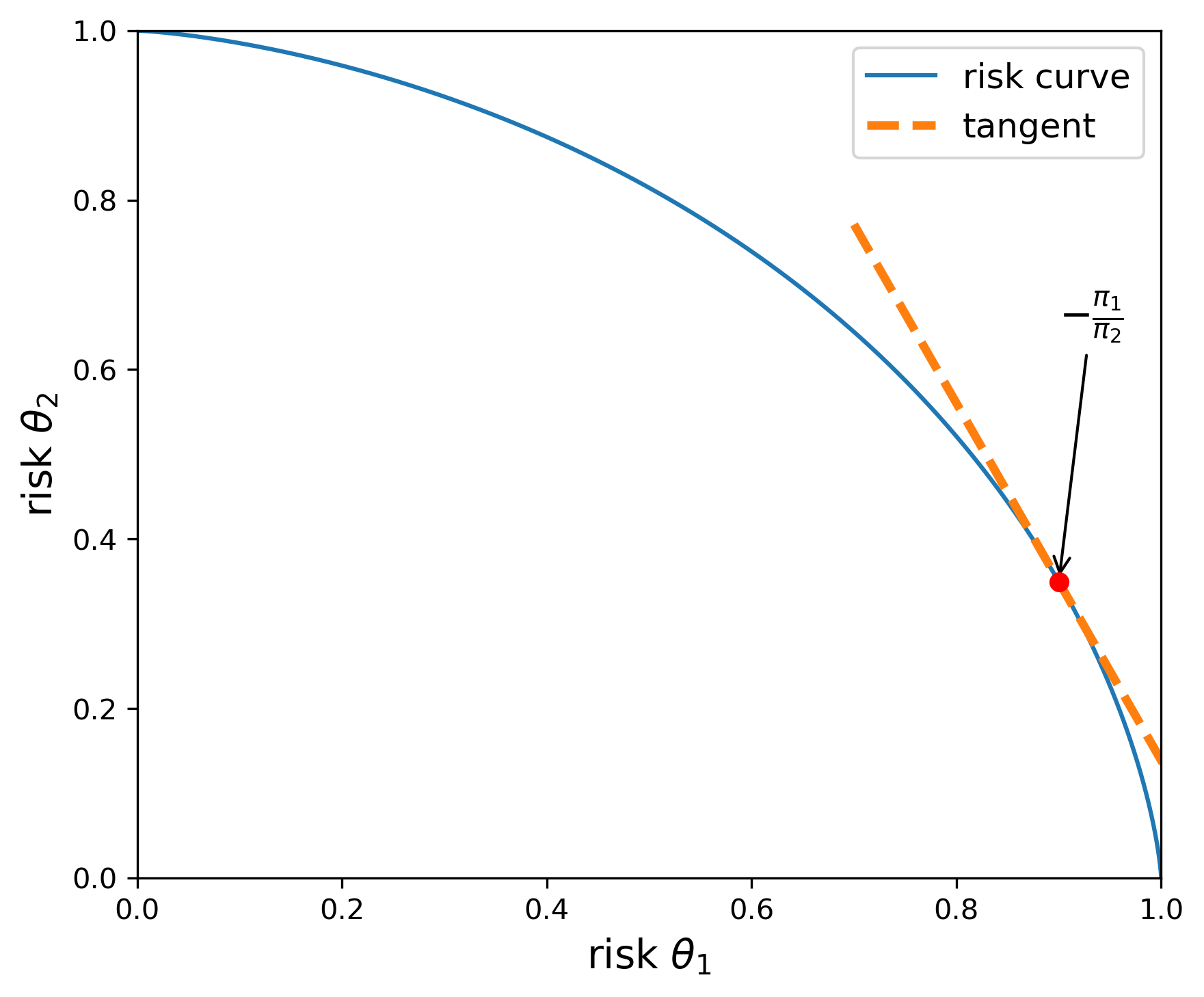
Fig. 10.1 The blue curve gives the upper boundary of the feasible set of risks. The utility function parameters are given by \(\upsilon_1=\upsilon_2=1.\) When \({\overline u}_{\sf r}(\theta_1) = .9\), the implied prior is given by \(\pi(\theta_1) =.68\) and \(\pi(\theta_2)=.32,\) as implied by the slope of the tangent line.#
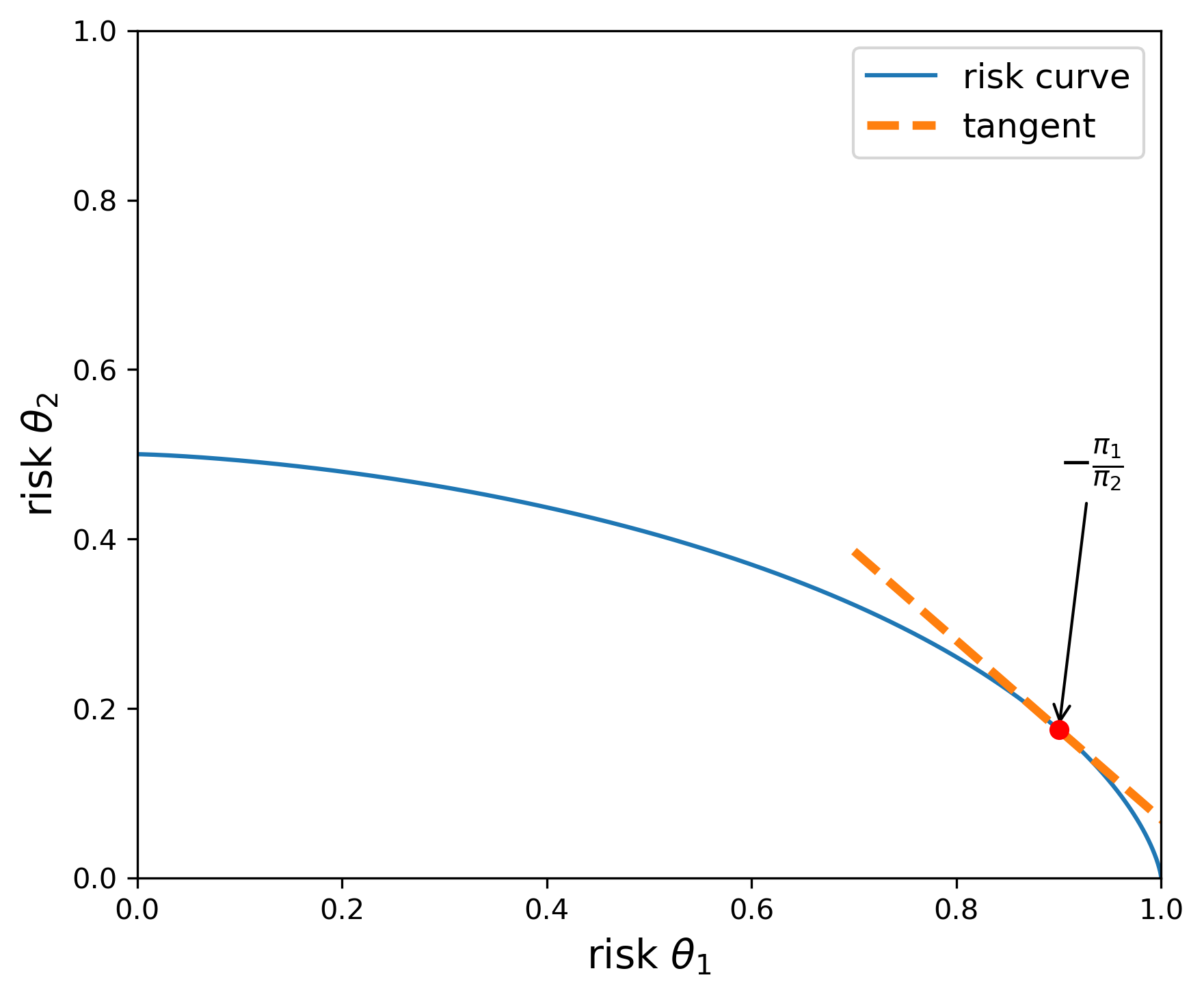
Fig. 10.2 The blue curve gives the upper boundary of the feasible set of risks. The utility function parameters are given by \(\upsilon_1= 1, \, \upsilon_2=.5.\) When \({\overline u}_{\sf r}(\theta_1) = .9\), the implied prior is given by \(\pi(\theta_1) =.51\) and \(\pi(\theta_2)=.49,\) as implied by the slope of the tangent line.#
10.6. Divergences#
To investigate prior sensitivity, we seek a convenient way to represent a family of alternative priors. We start with a baseline prior \(d \pi(\theta).\) Consider alternative priors of the form \(d \pi(\theta) = n(\theta) d\pi(\theta)\) for \(n \ge 0\) satisfying:
Call this collection \({\mathcal N}\). Thus the \(n\)’s in \({\mathcal N}\) are expressed as densities relative to a baseline prior distribution.
Introduce a convex function \(\phi\) to construct a divergence between a probability distribution represented by \(n \ne 1\) and the baseline probability. Restrict \(\phi\) to satisfy \(\phi(1) = 0\) and \(\phi''(1) = 1\) (normalization). As a measure of divergence, form
Of course, many such divergences can be constructed. Three interesting ones use the convex functions:
\(\phi(n) =- \log n\)
\(\phi(n) =\frac {n^2 -1}{2}\)
\(\phi(n) = n \log n\)
The divergence implied from the third choice is commonly used in applied probability theory and information theory. It is called Kullback-Leibler divergence or relative entropy. More generally, divergences for alternative choices of \(\phi\) are called \(\boldsymbol{\phi}\)-divergences or f-divergences.
10.7. Robust Bayesian preferences and ambiguity aversion#
Since the Bayesian ranking of prize rules depends on the prior distribution, we now explore how to proceed if the decision maker does not have full confidence in a specific prior. This leads naturally to an investigation of prior sensitivity. A decision or policy problem provides us with an answer to the question: sensitive to what. One way to investigate prior sensitivity is to approach it from the perspective of robustness. A robust decision rule then becomes one that performs well under alternative priors of interest. To obtain robustness guarantees, we are naturally led to minimization, providing us with a lower bound on performance. As we will see, prior robustness has very close ties to preferences that display ambiguity aversion. Just as risk aversion induces a form of caution in the presence of uncertain outcomes, ambiguity aversion induces a caution because of the lack of confidence in a single prior.
We explore prior robustness by using a version of variational preferences ([Maccheroni et al., 2006])
for \(\xi_1 > 0\) and a convex function \(\phi_1\) such that \(\phi_1(1)= 0\) and \({\phi_1}''(1) = 1.\) The penalty parameter \(\xi_1\) reflects the degree of ambiguity aversion. An arbitrarily large value of \(\xi_1\) approximates subjective expected utility. Relatively small values of \(\xi_1\) induce relatively large degrees of ambiguity aversion.
Remark 10.2
Axiomatic developments of decision theory in the presence of risk typically do not tell us the functional form for the utility function. Doing that requires additional inputs. An analogous observation applies to the axiomatic development of variational preferences by [Maccheroni et al., 2006]. Their axioms do not inform as to how to capture the cost associated with search over alternative priors.
Remark 10.3
The variational preferences of [Maccheroni et al., 2006] also include preferences with a constraint on priors:
The more restrictive axiomatic formulation of [Gilboa and Schmeidler, 1989] supports a representation with a constraint on the set of priors. In this case we use standard Karush-Kuhn-Tucker multipliers to model the preference relation:
10.7.1. Preferences with relative entropy divergence#
Suppose we use \(n \log n\) to construct our divergence measure. Recall the construction of the risk function
Solve the Lagrangian:
This problem separates in terms of the choice of \(n(\theta)\), and can be solved \(\theta\) by \(\theta\). The first-order conditions are:
Solving for \(\log n(\theta)\):
Thus
Imposing the integral constraint on \(n\) gives the solution:
provided that the denominator is finite. This solution induces what is known as exponential tilting. The baseline probabilities are tilted towards lower values of \({\overline { U}}(\gamma \mid \theta)\). Plugging back into the minimization problem gives:
This minimized objective is known to be a special case of smooth ambiguity preferences initially proposed by [Klibanoff et al., 2005], although these authors provide a different motivation for their ambiguity adjustment. The connection we articulate opens the door to a more direct link to challenges familiar to statisticians and econometricians wrestling with how to analyze and interpret data. Indeed [Cerreia-Vioglio et al., 2013] also adopt a robust statistics perspective when exploring smooth ambiguity aversion preferences. They use constructs and distinctions of the type we explored in Chapter 1 in characterizing what is and is not learnable from the Law of Large Numbers.
10.7.2. Robust Bayesian decision problem#
We extend Decision Problem (10.1) to include prior robustness by introducing a special case of a two-player, zero-sum game:
Game 11.4
Notice that in this formulation, the minimization depends on the choice of the prize rule \(\gamma\) and hence on the decision rule \(\delta\) that constrains \(\gamma\). This is to be expected as the prior with the most adverse consequences for the expected utility should plausibly depend on the potential course of action under consideration.
For a variety of reasons, it is of interest to investigate a related problem in which the order of extremization is exchanged:
Game 11.5
Notice that for a given \(n\), the inner problem is essentially just a version of the Bayesian problem (10.1). The penalty term
is additively separable and does not depend on \(\delta\). In this formulation, we solve a Bayesian problem for each possible prior, and then minimize over the priors taking account of the penalty term. Provided that the outer minimization problem over \(n\) has a solution, \(n^*,\) the implied decision rule, \(\delta_{n^*},\) solves a Bayesian decision problem. As we know from section Constructing admissible decision rules, this opens the door to verifying admissibility.
The two decision games, (10.11) and (10.12), essentially have the same solution under a Minimax Theorem. That is the implied value functions are the same and \(\delta_{n^*},\) from Game (10.12) solves Game (10.11) and gives the robust decision rule under prior ambiguity. This result holds under a variety of sufficient conditions. Notice that the objective for Game (10.11) is convex in \(n\). A well known result due to [Fan, 1952] verifies the Minimax Theorem when the objective satisfies a generalization of concavity with a convex constraint set \(\Delta\). While we cannot always justify this exchange, there are other sufficient conditions that are also applicable.
A robust Bayesian advocate along the lines of [Good, 1952], views the solution, say \(n^*,\) from Game (10.12) as a choice of a prior to be evaluated subjectively. It is often referred to as a “worst-case prior”, but an object that is of interest in its own right. For an application of this idea in economics see [Chamberlain, 2000].[6] Typically, \(n^*(\theta) d\pi(\theta)\) can be computed as part of an algorithm for finding a robust decision rule, and is arguably worth serious inspection. While we could just view robustness considerations as a way to select a prior, the (penalized) worst-case solutions can instead be viewed as a device to implement robustness. While they are worthy of inspection, just as with the baseline prior probabilities, the worst-case probabilities are not intended to be a specification of a fully confident input of subjective probabilities and are dependent on the utility function and constraints imposed on the decision problem.
10.7.2.1. A simple application reconsidered III#
We again use the model selection example to illustrate ambiguity aversion in the presence of a relative entropy cost of a prior deviating from the baseline. Since the Minimax Theorem applies, we focus our attention on admissible decision rules parameterized by thresholds of the form (10.8). With this simplification, we use formula (10.10) and solve the scalar maximization problem:
This maximization problem may be solved easily using a numerical method. Nevertheless, the first-order conditions are:
Notice the exponential tilting adjustment to the prior probabilities. The resulting threshold decision rule is admissible, which can be verified using these altered probabilities. The first-order conditions can be further simplified to
We consider two limiting cases. When \(\xi_1 \rightarrow \infty\), the first two terms drop out and the first-order conditions are the ones for maximizing the subjective expected utility:
To investigate the solution when \(\xi_1 \rightarrow 0\), we first multiply (10.13) by \(\xi_1\) in advance of taking the limit. The result
Thus the robustly optimal \({\sf r}\) is determined by making the two possible risks equal.
For a more general decision rule, \(\delta\), form the two risks:
The minimization in this limiting case assigns probability one to lowest risk with an objective:
Graphically, the objective for any point to the left of the 45 degree line from the origin equals the outcome of a vertically downward movement to that same line. Analogously, the objective for any point to the right of the 45 degree line from the origin equals the outcome of a horizontally leftward movement to that same line. Thus the maximizing \(\delta\) is obtained at the intersection of the 45 degree line and the boundary of the risk set. Along the 45 degree line, the choice of prior is inconsequential because the two risks are the same. Nevertheless, the “worst-case” prior is determined by slope of the risk curve at the intersection point. Recall that we defined this prior after exchanging orders of extremization. Figures Fig. 10.3 and Fig. 10.4 illustrate this outcome for the two risk curves on display in Figures Fig. 10.1 and Fig. 10.2.
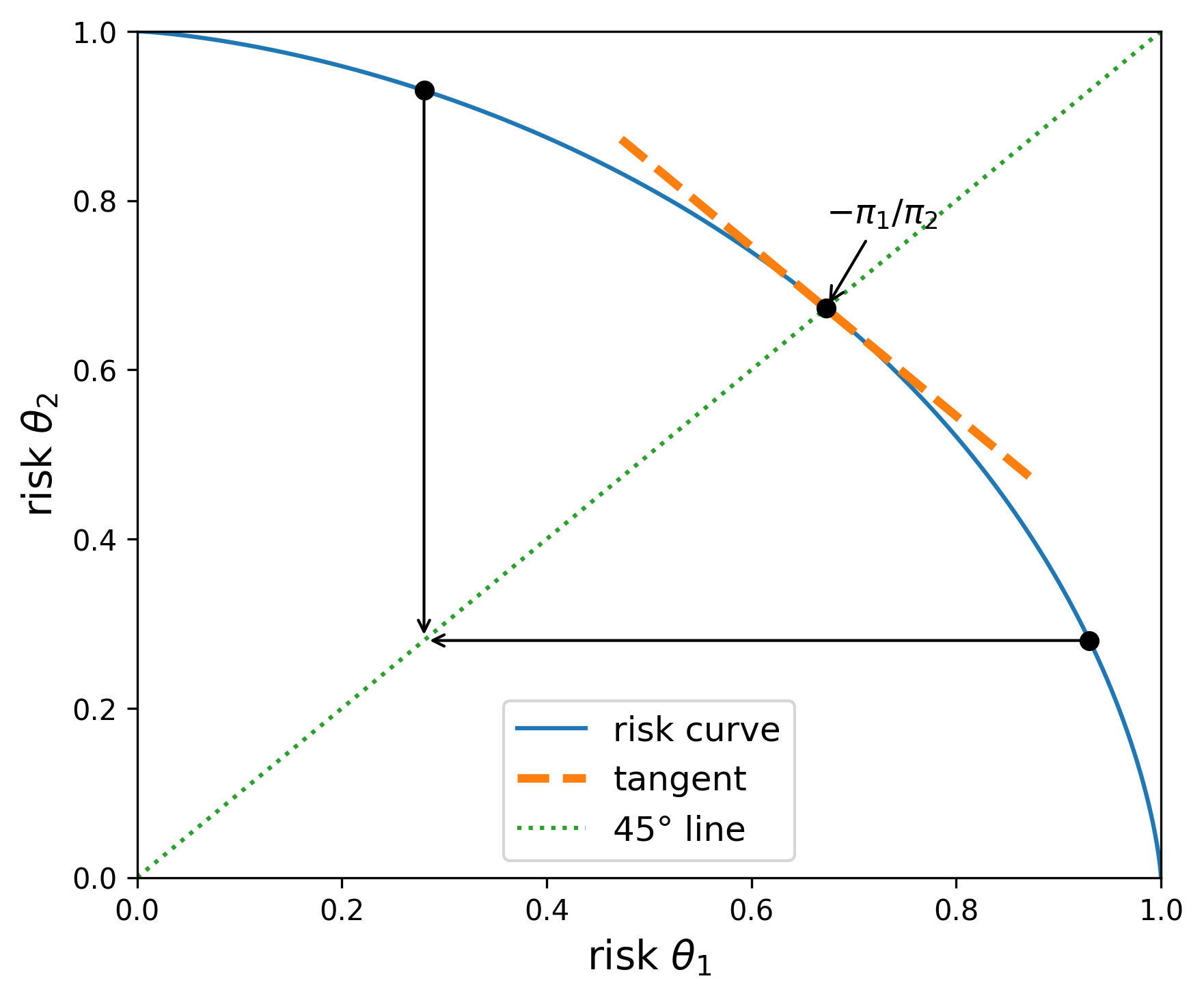
Fig. 10.3 The blue curve gives the upper boundary of the feasible set of risks. The utility function parameters are given by \(\upsilon_1=\upsilon_2=1.\) The implied worst-case prior is given by \(\pi(\theta_1) =.5\) and \(\pi(\theta_2)=.5,\) as implied by the slope of the tangent line at the intersection with the 45 degree line from the origin.#
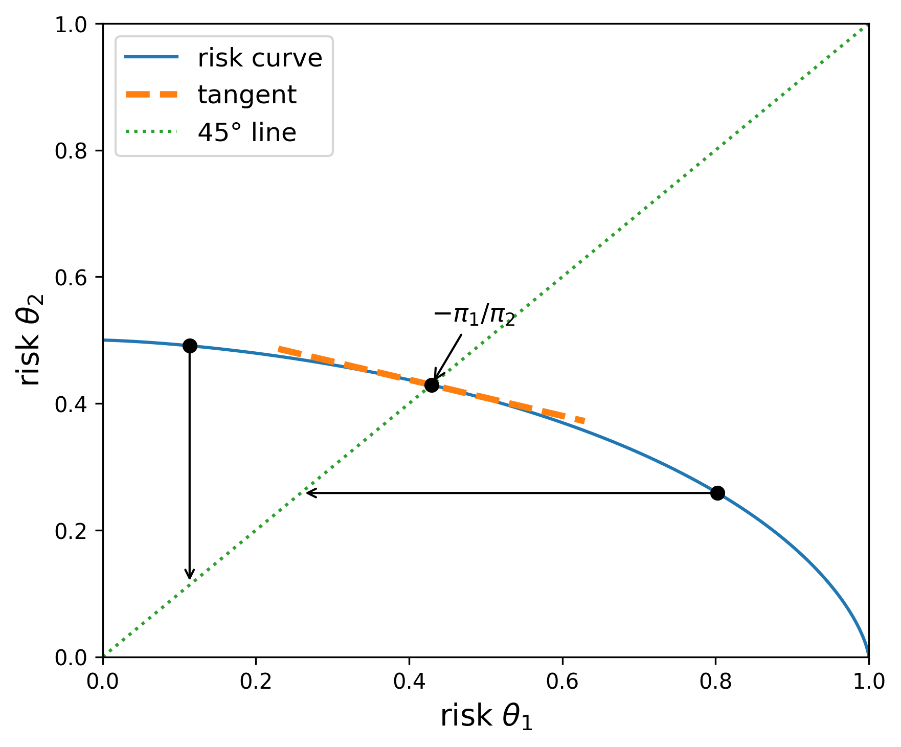
Fig. 10.4 The blue curve gives the upper boundary of the feasible set of risks. The utility function parameters are given by \(\upsilon_1=1\) and \(\upsilon_2=.5.\) The implied worst-case prior is given by \(\pi(\theta_1) =.22\) and \(\pi(\theta_2)=.78,\) as implied by the slope of the tangent line at the intersection with the 45 degree line from the origin.#
For positive values of \(\xi_1,\) the implied worst-case priors are between the baseline \(\pi\) (\(\xi = \infty\)) and the worst-case without restricting the prior probabilities (\(\xi = 0\)). Observe that the worst-case priors depend on the utility weights, \(\upsilon_1\) and \(\upsilon_2\). See Figures Fig. 10.5 and Fig. 10.6 as illustrations.
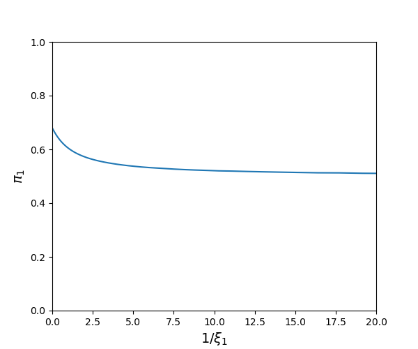
Fig. 10.5 Minimizing prior probabilities for \(\theta_1\) as a function of \(1/\xi_1\) when the baseline prior probabilities are \(\pi(\theta_1) = .68\) and \(\pi(\theta_2) = .32\) and the utility parameters are \(\upsilon_1=\upsilon_2=1.\)#
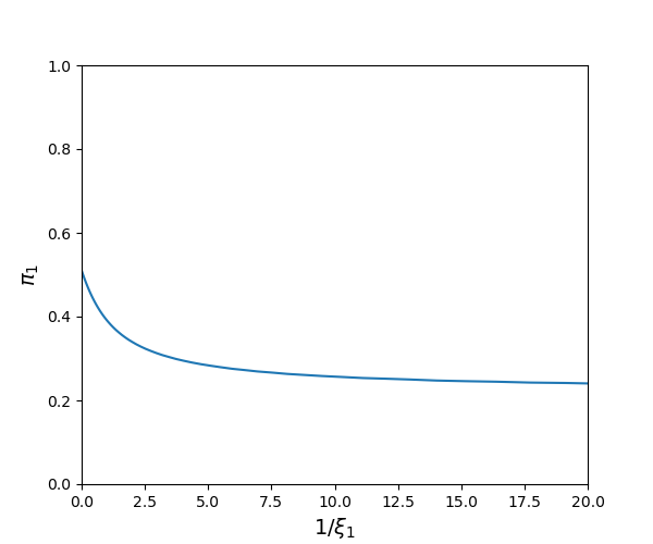
Fig. 10.6 Minimizing prior probabilities for \(\theta_1\) as a function of \(1/\xi_1\) when the baseline prior probabilities are \(\pi(\theta_1) = .51\) and \(\pi(\theta_2) = .49\) and the utility parameters are \(\upsilon_1= 1\) and \(\upsilon_2=.5.\)#
The model selection example dramatically understates the potential value of ambiguity aversion as a way to study prior sensitivity. In typical applied problems, the subjective probabilities are imposed on a much richer collection of alternative models including families of models indexed by unknown parameters. In such problems the outcome is more subtle since the minimization isolates dimensions along which prior sensitivity has the most adverse impacts on the decision problem and are perhaps most worthy of further consideration. This can be especially important in problems where baseline priors are imposed “as a matter of computational convenience.”
10.8. Using uncertainty aversion to represent concerns about model misspecification#
Two prominent statisticians remarked on how model misspecification is pervasive:
“Since all models are wrong, the scientist must be alert to what is importantly wrong. It is inappropriate to be concerned about mice when there are tigers abroad.” — Box (1976).
“… it does not seem helpful just to say that all models are wrong. The very word ‘model’ implies simplification and idealization. The idea that complex physical, biological or sociological systems can be exactly described by a few formulae is patently absurd. The construction of idealized representations that capture important stable aspects of such systems is, however, a vital part of general scientific analysis and statistical models, especially substantive ones …” — Cox (1995).
Other scholars have made similar remarks. Robust control theorists have suggested one way to address this challenge, an approach that we build on in the discussion that follows. Motivated by such sentiments, [Cerreia-Vioglio et al., 2025] extended decision theory axioms to accommodate misspecification concerns. To proceed, we focus our analysis of model misspecification by conditioning on \(\theta.\) Our decision maker will no longer have full confidence in the probability specification \(\ell(x \mid \theta) d\tau(x).\) In other words, our treatment of this probability is no longer as a source of risk, or as a “roulette wheel” lottery in the sense of [Anscombe and Aumann, 1963]. Instead of exploring sensitivity to probability specifications over a parameter space \(\Theta,\) our focus shifts to exploring sensitivity to alternative probability specifications over the space \({\mathcal X}\) for which \(\ell(x \mid \theta) d\tau(x)\) merely serves as baseline. Think of this baseline as implied by a model of interest. We then consider alternative probability assignments to entertain potential model misspecification.
10.8.1. Basic approach#
To focus on the misspecification of a specific model, we fix \(\theta\), but vary the likelihood function as a way to investigate likelihood sensitivity. We then replace \(\ell\) with \(m \ell \) satisfying:
and denote the set of all such density ratios \(m\) as \(\mathcal M\).
Observe that \(m(x \mid \theta)\) can be viewed as the ratio of two densities. Consider two alternative probability densities (with respect to \(d \tau(x)\)) for shock/signal probabilities: \(\ell(x \mid \theta)\) and \({\tilde \ell}(x \mid \theta)\) and let:
where we assume \(\ell(x \mid \theta) > 0\) for \(x \in {\mathcal X}\). Then by construction:
and
We use density ratios to capture alternative models as inputs into divergence measures. Let \(\phi_2\) be a convex function such that \({\phi_2}(1) = 0\) and \({\phi_2}''(1) = 1\) (normalization). Instead of specifying a divergence between probabilities over the parameter space, \(\Theta,\) we now impose the divergence over the \({\mathcal X}\) space:
We use this divergence to limit or constrain our search over alternative probability models. In this approach we deliberately avoid imposing a prior distribution over the space of densities (with respect to \(d \tau(x)\)).
Preferences for model robustness rank alternative prize rules, \(\gamma\), by solving:
for a penalty parameter \(\xi_2 > 0.\) The parameter, \(\xi_2\), dictates the strength of the restraint in an exploration of possible model misspecifications.
10.8.2. Relative entropy divergence#
This approach to model misspecification has direct links to robust control theory in the case of relative entropy divergence. Suppose that \(\phi_2(m) = m \log m\) (relative entropy). Then by imitating previous computations, we find that the outcome of the minimization in (10.14) is
Remark 10.4
Robust control emerged from the study of optimization of dynamical systems. The use of the relative entropy divergence showed up prominently in [Jacobson, 1973] and later in [Whittle, 1981], [Petersen et al., 2000] and many other related papers as a response to the excessive simplicity of assuming shocks to dynamical systems that were iid and mean zero with normal distributions. [Hansen and Sargent, 1995] and [Hansen and Sargent, 2001] showed how to reformulate the insights from robust control theory to apply to dynamical economic systems with recursive formulations and [Hansen et al., 1999] used these ideas in an initial empirical investigation.
When we use relative entropy as a measure of divergence, we have the ability to factor likelihoods in convenient ways. Recall the partitioning \(x = (w, z)\), where the decision rule can only depend on \(z\) and the prize rule on the entire \(x\) vector. As in (10.2), factor \(\ell(\cdot \mid \theta)\) and \(\tau\) as:
Add to this a factorization of \(m(\cdot \mid \theta)\),
Let \({\mathcal M}_1\) denote the set of \(m_1(z \mid \theta) \ge 0\) that satisfy the relevant integral constraint in (10.15), and similarly let \({\mathcal M}_2\) be the set of \(m_2(w \mid z, \theta) \ge 0\) that satisfy the relevant integral constraint.
Using these factorizations, the relative entropy may be written as:
where the first contribution features the potential misspecification of the conditional probability over \({\mathcal W}\) and the second term features the potential misspecification of the probability over \({\mathcal Z}.\)
Rewrite the expected utility function in (10.14) with an inner integral:
Notice that both the formulas (10.16) and (10.17) scale linearly in \(m_1(z \mid \theta)\) and that the additional relative entropy term depends only on \(z\). Thus we can use a conditional objective when solving for robust decision rule \(\delta\):
Game 11.6
where constraint set \(\Delta\) satisfies the separability constraint (10.3).
Notice that the minimizing over \(m_1\) does not play a role in constructing a robustly optimal decision in this setup since the decision rule can depend on what value of \(z\) is realized.
Remark 10.5
Rather than conditioning on a parameter value, [Chamberlain, 2020] argues for exploring the potential misspecification of the so called predictive density. Given a baseline probability density over \({\mathcal X}\) conditioned on a parameter vector and a baseline prior over the family \(\Theta\) of potential models, form a density over ${\mathcal X}
Use this single density over \({\mathcal X}\) as the basis for a robustness adjustment. In what follows we explore approaches that treat potential prior misspecification and model misspecification as distinct concerns.
Remark 10.6
It is useful to compare two approaches to robustness that we have taken. One possibility is that the decision maker starts with a baseline prior over parameter vectors and considers consequences of misspecifying that prior. Under this approach, the decision maker takes as given the parameterized family of densities, \(\ell(x \mid \theta)\) that imply a corresponding parameterized family of probabilities over the set of parameter \(\Theta\)’s as correctly specified. As an alternative, instead of parameterizing a family of densities, suppose we start with one such density and explore its potential misspecification.
Our setup allows the parameter space to be infinite dimensional. Consider a prior that is consistent with a “nonparametric Bayesian approach to decision making.” Specifying a prior over the infinite-dimensional space exposes a challenge associated with “nonparametric Bayesian” methods. The prior probability must assign probability one to what is called a “meager set.” A meager set is defined topologically as a countable union of nowhere dense sets and is arguably small within an infinite-dimensional space. See [Freedman, 1963], [Sims, 1971], and [Diaconis and Freedman, 1986] for formal elaborations. This conclusion carries over to situations with families of priors that are absolutely continuous with respect to a baseline prior, as we have here. To us, prior robustness of this form is interesting, although it is distinct from robustness to the potential misspecification of a probability distribution on \({\mathcal X}.\)
10.9. Robust Bayes with model misspecification#
So far we have explored two misspecification concerns in separate formulations. We now explore the potential misspecification of \(\ell(x \mid \theta) d\tau(x) \) simultaneously with a prior \(\pi\) over the parameters.
It requires a different decision theory perspective as developed recently in [Cerreia-Vioglio et al., 2025]. Their contribution was motivated by earlier contributions [Hansen and Sargent, 2007] and [Hansen and Sargent, 2022] that proposed representations without formal axiomatic defenses. The latter paper presents a class of continuous-time diffusion models for which the robustness distinction between likelihood and prior potential misspecification is captured by featuring a set of “structured” models that could each be misspecified.
10.9.1. A modified decision theory formulation#
Combining concerns for likelihood and prior misspecification pushes the decision problem outside the Savage and Anscombe-Aumann frameworks. [Cerreia-Vioglio et al., 2025] recently proposed an extension of the Anscombe-Aumann formulation. Their advance was motivated by earlier contributions [Hansen and Sargent, 2007] and [Hansen and Sargent, 2022] that proposed representations of decision problems, but they did not provide an axiomatic defense for these representations. The latter paper presents a class of continuous-time diffusion models for which the robustness distinction between model and prior potential misspecification is captured by featuring a set of “structured” models, each of which could be misspecified.
[Cerreia-Vioglio et al., 2025] incorporate a two-preference framework proposed previously by [Gilboa et al., 2010]. One of the preferences is referred to as “mental preferences.” These preferences are incomplete and only provide a partial ordering induced by unanimity over all structured models. We saw an analogous approach in our treatment of admissibility. Whereas we defined admissibility in terms of risk functions, we allow the mental preferences to incorporate model misspecification concerns of the type that we analyzed in the previous section. We then construct “behavioral preferences” that are complete and used in actual decision making by entertaining ambiguity aversion over structured probability models. [Cerreia-Vioglio et al., 2025] provide a formal axiomatic defense for proceeding in this fashion. What follows are two approaches that can be accommodated within this extended decision theory.
10.9.2. Approach one#
Form a convex, compact constraint set of prior probabilities, \( {\mathcal N}_o \subset {\mathcal N}\). Represent preferences over \(\gamma\) using:
This is a special case of what [Gilboa and Schmeidler, 1989] call “max-min expected utility” with a nonunique prior.
10.9.3. Approach two#
Represent preferences over \(\gamma\) using:
Note that this approach uses a scaled version of a joint divergence over \((m,n),\) as reflected in the term
Either can be used when formulating decision problems. For instance, the associated decision problem for the second approach is:
Game 11.7
Remark 10.7
Consider the special case in which \(\xi_1 = \xi_2 = \xi,\) and use this common parameter to scale a relative entropy divergence. Then the combined robustness penalty contribution to preferences is measured by \(\xi\) multiplying the relative entropy of the joint distribution \(m(x \mid \theta) n(\theta) \ell(x \mid \theta) d\tau(x) d\pi(\theta) \) relative to the baseline \(\ell(x \mid \theta) d\tau(x) d\pi(\theta)\) and given by:
Joint densities can be factored in alternative ways. In solving the robust decision problem, a different factorization is more convenient that conditions on the data available for making decisions. As we have done previously, form three contributions of the joint density under the baseline:
Notice that the last term in the factorization depends only on \(z,\) whereas the decision rule conditions on \(z.\) We now explore likelihood misspecification using \(m_2(w \mid z, \theta)\) satisfying:
and posterior misspecification using \({\bar n}(\theta \mid z )\) where
Thus to compute \(\delta\) we again have a type of separation where we alter the posterior implied by the baseline probability specifications and the conditional density for \(\ell_2(w \mid z, \theta)\). We may alter the density
in an analogous way, but this exploration will have no impact on the robustly optimal choice of \(\delta\).
The logic behind this conditioning is entirely analogous to the argument we provided for the conditional version of the Bayesian decision problem. The objective for the conditional robust game is:
Game 11.8
where constraint set \(\Delta\) satisfies the separability constraint (10.3).
If the utility function does not depend directly on \(\theta,\) we may perform the robustness analysis on a conditional version starting with the predictive density over \({\mathcal W}\)
which is a conditional version of the proposal in [Chamberlain, 2020].
While \(\xi_1= \xi_2\) opens the door to computing robustly optimal decision rules via conditioning, we find this penalty equalization to be too constraining for many problems of interest. For example, [Hansen and Miao, 2018] describe continuous environments for which it is important that \(\xi_1 \ne \xi_2.\)
10.10. A dynamic robust decision problem under commitment#
So far, we have studied static decision problems. This formulation can accommodate dynamic problems by allowing for decision rules that depend on histories of data available up until the date of the decision. To convert to a static problem we pose the corresponding two-player game as one with a date zero “commitment” to robustly optimal decision rules at the initial date.
Recall from Chapter 1 that we use an ergodic decomposition to identify a family of statistical models that are dynamic in nature, along with probabilities across models that are necessarily subjective as they are not revealed by data. The example incorporates this perspective.
Consider the following example of a real investment problem with a single stochastic option for transferring goods from one period to another. This problem could be a planner’s problem supporting a competitive equilibrium outcome associated with a stochastic growth model with a single capital good. Introduce an exogenous stochastic technology process that has an impact on the growth rate of capital. We design this stochastic technology process to capture what a previous literature in macro-finance has referred to as “long-run risk.” For instance, see [Bansal and Yaron, 2004].[7]
We extend this formulation by introducing a parameterized family of stochastic technology processes. This gives rise to a family of “structured models”. The investor’s exploration of the entire family of these processes reflects uncertainty among possible structured models. We also allow the investor to entertain misspecification concerns for each of the structured models.
The exogenous (system) state vector \(Z_{t}\) is used to capture fluctuations in technological opportunities, and \(W_{t+1}\) is a bi-variate, standard, normally distributed shock vector. We build the exogenous technology process from the shocks in a parameter-dependent way:
for a given initial condition \(Z_{0}\).
For instance, in long-run risk modeling one component of \(Z_{t}\) evolves as a first-order autoregression:
and another component is given by:
The matrix: \( [{\mathbf b}_\theta^1 \hspace{.3cm} {\mathbf b}_\theta^2] \) is presumed to be nonsingular for all values of \(\theta\).
At each time \(t\) the investor observes past and current values \(\mathbf{Z} ^{t}=\left \{ Z_{0},Z_{1},...,Z_{t}\right \} \) of the technology process, but does not know \(\theta\) and does not directly observe the random shock vector \(W_{t}\).
Similarly, we consider a recursive representation of capital evolution given by:
where \(\varphi\) is used to capture adjustment costs for changing the capital stock. Consumption \(C_{t}\geq0\) and investment \(I_{t}\geq0\) are constrained by an output relation:
for a pre-specified initial condition \(K_{0}\). The parameter \(\alpha\) captures the productivity of capital. By design this technology is homogeneous of degree one, which opens the door to stochastic growth as assumed in long-run risk models. In what follows we let the date \(t\) decision variable be:
Then \(C_t/K_t\) is constrained by
Thus date \(t\) consumption, \(C_t,\) can be inferred from \(D_t\) and \(K_t\). While preferences are defined over consumption processes, we express the date \(t\) contribution to the discounted utility as a function of \(D_t\) and \(K_t\). The date \(t\) decision \(D_t\) is constrained to be a function of \(\mathbf{Z}^{t}\) at each date \(t\), reflecting the observational constraint that \(\theta\) is unknown to the investor in contrast to the history \(\mathbf{Z}^{t}\) of the technology process.[8] Let \({\mathfrak B}_t\) be the collection of events (sigma algebra) generated by \(\mathbf{Z}^t\) and \(K_0\). We denote the larger sigma algebra that also conditions on knowledge of the parameter to be \({\mathfrak B}_t^+.\)
Absent robustness concerns the preferences are given by
We include divergences, one for the prior on the set of possible parameter values, \(\Theta,\) and the other for the potential misspecification in the dynamics as reflected in the shock distributions. The latter divergence will necessarily be dynamic in nature. We introduce a positive martingale \(\{ M_t : t \ge 0 \}\) for an altered probability. Let \(M_0=1\) and let \(M_t\) be measurable with respect to \({\mathfrak B}_t^+.\) We use the random variable \(M_t\) to alter date \(t\) probabilities conditioned on \({\mathfrak B}_0^+\) when evaluating the discounted expected utility:
Construct an intertemporal divergence:
as a measure of divergence and scale this by a penalty parameter, \(\xi_2\). We purposefully discount the relative entropies in the same way as we discount the utility function, and the computations are conditioned on \(\theta\). We then use a second divergence to investigate prior sensitivity over the space of potential parameter vectors \(\theta\) with a penalty parameter \(\xi_1.\)
In this model, the investor or planner will use available data to learn about \(\theta\) at each point in time. By contrast, the potential model misspecifications are presumed not to be learnable because the formulation allows for potential departures at future dates to be different from those that might have been present in the past. This model formulation allows for a lack of confidence in both the prior and intertemporal state dynamics.
10.11. A recursive counterpart to a dynamic robust decision problem#
10.11.1. Model misspecification concerns#
To construct a recursive formulation of preferences, we first deduce a recursive representation of the model misspecification divergence measure by exploiting the multiplicative martingale construction. Let \(\{ {\mathfrak B}_t: t \ge 0\}\) capture the decision maker information available at the respective dates. In our focus on misspecification concerns, we condition on the parameter \(\theta\). Write:
and \(M_0\) is initialized to be one. By the Law of Iterated Expectations:
Using this calculation and applying “summation-by-parts” (implemented by changing the order of summation) gives:
In this formula,
is the relative entropy pertinent to the transition probabilities between date \(t\) and \(t+1\). Abstracting from parameter uncertainty, given this recursive structure, we may evaluate the objective and solve the decision problem recursively. The recursive and commitment solutions will coincide which opens the door to the use of dynamic programming methods.
Using representation (10.21) as input, we construct a recursive representation for preferences over decision processes. Specifically, an implied recursion for the robust-adjusted continue values
where \(V_t(k)\) is the current-period continuation value as a function of the possible values for the date \(t\) capital stock. The ratio \(M_{t+1}/M_{t}\) is used when computing the conditional expectation of next period’s continuation value, \(V_{t+1}\). In forming this recursion, we substituted the right-hand side of capital evolution equation (10.19) for \(K_t=k\) into the next period continuation value. Imitating our previous computations, we substitute a solution of the minimization contribution to obtain:
Notice that this recursion is essentially the same as that we introduced in Chapter 4. (See (4.8).) The rationale provided here is the decision-maker concern about model misspecification instead of risk aversion.
With preference recursion, (10.22) we can apply dynamic programming methods to compute a robustly-optimal control by solving:
the recursion:
In this formulation, we have assumed knowledge of the parameter \(\theta.\) While the maximizing \(D_t\) will be \({\mathfrak B}_t^+\) measurable, it will typically not be \({\mathfrak B}_t\) measurable.
Remark 10.8
Our discounting of relative entropy has important consequences for exploration of potential misspecification. From (10.20), it follows that the sequence
is increasing in \(t\). Observe that
gives an upper bound on
for each \(s \ge 0\). This follows from monotonicity since
Taking limits as \(\beta \uparrow 1\) gives the bound of interest.
If the discounted limit in (10.25) is finite, then the increasing sequence (10.24) has a finite limit. It follows from a version of the Martingale Convergence Theorem (see [Barron, 1990]) that there is a limiting random nonnegative variable \(M_\infty\) such that \(E \left( M_\infty \mid {\mathfrak B}_0^+ \right) =1\) and
When the limiting random variable, \(M_\infty,\) is well defined, almost sure limits under the probability specification must agree with those under the change implied probability measure induced by \(M_\infty.\) If the limiting random variable is strictly positive, then the baseline and the \(M_\infty\) imply the same Law of Large Numbers. In this sense, only transient departures from the baseline probability are part of the misspecification exploration. By including discounting, we expand the family of alternative probabilities in a substantively important way.
As an alternative calculation, consider a different discount factor scaling:
The limiting version of this measure allows for a substantially larger set of alternative probabilities and results in a limiting characterization that is used in Large Deviation Theory as applied in dynamic settings.
Remark 10.9
To explore potential misspecification [Eckstein, 2019] and [Chen et al., 2020] suggest other divergences with convenient recursive structures. A discounted version of their proposal is
for a convex function \(\phi_2\) where this function equals one when evaluated at one, and its second derivative at one is normalized to be one.
10.11.2. A recursive formulation with parameter ambiguity#
Once we include parameter uncertainty, we lose the recursive structure in the commitment version of the decision problem. We now suggest a recursive specification of preferences that includes parameter uncertainty, but with distinct preferences from those used for the commitment problem.
Let \(N_t \ge 0\) be a scalar random variable that is \({\mathfrak B}_t^+\) measurable and satisfies:
Recall that we constructed \({\mathfrak B}_t^+\) to include knowledge of the underlying parameter vector in contrast to \({\mathfrak B}_t.\) A “behind the scenes” recursive learning input will be needed to implement computations based on the smaller sigma algebra \({\mathfrak B}_t\) in what follows. We use \(N_t\) to alter baseline date \(t\) expectations by altering the posterior probabilities over the possible unknown parameters, but those posteriors typically require recursive computations of the type we illustrated in Chapter 5.
We now incorporate parameter learning into recursion (10.22) for ranking alternative decision processes
Analogously, we modify recursion (10.23) used for finding the robustly optimal decision processes:
The solution for \(D_t\) will be \({\mathfrak B}_t\) measurable, which excludes knowledge of the parameter vector. This formulation gives a dynamic extension of Game 11.6.
Remark 10.10
Consider the special case in which \(\xi_1 = \xi_2\) and \(\phi_1(n) = n\log n\). In this case we are essentially using a single divergence over a joint density. We may imitate previous logic and apply a single robust adjustment expressed in terms of the transition probabilities from \({\mathfrak B}_{t}\) to \({\mathfrak B}_{t+1}\) in place of recursions used in (10.22) and (10.23). The exploration supporting robustness in both transition dynamics and the date \(t\) distribution over the parameter \(\theta\) led us to use:
to induce a change in probabilities conditioned on \({\mathfrak B}_t\). As an alternative to using this factorization, we now explore the ramifications of a different one by writing:
Observe the composite divergence used in defining preferences can be expressed equivalently with the two different factorizations:
The right-hand side of the first equality is what we have used in constructing penalties for model misspecification concerns and ambiguity over alternative models. The right-hand-side of the third equality leads to a simplification in the minimization problem. The continuation-value functions at date \(t+1,\) \(V_{t+1}(k)\) and \({\overline V}_{t+1}(k)\) are measurable with respect to \({\mathfrak B}_{t+1}\) and do not depend on the unknown \(\theta\). Thus the term:
will be set equal to one via minimization. In other words.
The relevant choice variable to use in minimization is the single contribution:
which, by construction, is \({\mathfrak B}_{t+1}\) measurable and has an expectation conditioned on \({\mathfrak B}_t\) that is equal to one. This random variable is used to alter the probabilities of \({\mathfrak B}_{t+1}\) events conditioned on \({\mathfrak B}_t\). In summary, for the robustness analysis over state dynamics and distributions over parameters, it suffices to focus on the minimization implications of such random variables subject to the corresponding relative entropy penalty. To implement this reduction in practice requires as input the recursive solutions to parameter learning under a baseline specification.
We do not take this argument as a blanket endorsement for the resulting simplification. Quite the contrary, we find it advantageous to explore the distinct roles of model misspecification and prior/posterior misspecification.
10.12. Implications for uncertainty quantification#
Uncertainty quantification is a challenge that pervades many scientific disciplines. The methods we describe here open the door to answering the “so what” aspect of uncertainty measurement. So far, we have deliberately explored examples that are low-dimensional to illustrate results. While these are pedagogically revealing, the methods we describe have all the more potency in problems with high-dimensional uncertainty. By including minimization as part of the decision problem, we isolate the uncertainties that are of most relevance to the decision or policy problem. This may pave the way for incorporating sharper prior inputs or for guiding future efforts aimed at providing additional evidence relevant to the decision-making challenge. Furthermore, there may be multiple channels by which uncertainty can impact the decision problem. As an example, consider an economic analysis of climate change. There is uncertainty in i) the global warming implications of increases in carbon emissions, ii) the impact of global warming on economic opportunities, and iii) the prospects for the discovery of new, clean technologies that are economically viable. A direct extension of the methods developed in this chapter provides a (non-additive) decomposition of the channels of uncertainty. By modifying the penalization, uncertainty in each channel could be activated separately in comparison to activating uncertainty in all channels simultaneously. Comparing outcomes of such computations reveals which channel of uncertainty is most consequential to the structuring of a prudent decision rule.[9]