11. Representing and Decomposing Marginal Valuations

Download PDF here

Authors: Lars Peter Hansen (University of Chicago) and Thomas J. Sargent (NYU)

\(\newcommand{\eqdef}{\stackrel{\text{def}}{=}}\)

“It thus becomes important to inquire in what conditions the values of the social net product and the private net product of any given increment … of investment … are liable to diverge from one another….” —Pigou (1920), The Economics of Welfare, Chapter IX

“If man is not to do more harm than good in his efforts to improve the social order, he will have to learn that in this, as in all other fields where essential complexity of an organized kind prevails, he cannot acquire the full knowledge which would make mastery of the events possible.” —Hayek (1974), Pretense of Knowledge

11.1. Introduction

Because partial derivatives of value functions appear in first-order conditions for controls in Markov decision problems, they can be used to measure marginal valuations. Such marginal valuations indicate directions for improving values and also losses that arise from making choices that are suboptimal from the perspective of a baseline controlled Markov process used to pose a Markov decision problem. Consequently, these marginal valuations also play an important role in max–min formulations of robust control. They are relevant for both individual decision problems and evaluations of social policies involving taxation and regulations affecting both physical and social environments. Within macroeconomics, robust-control theories have been used by [Hansen et al., 1999] to assess impacts of uncertainty on investment and equilibrium prices and quantities, and by [Alvarez and Jermann, 2004] to evaluate the welfare consequences of uncertainty, extending [Lucas, 1987]. In public economics, [Dasgupta and Mäler, 2001] apply marginal valuation to assess environmental capital and to ascertain directions of potential policy improvements. Thus, there is an extensive literature measuring the social cost of carbon with different approaches. See, for instance, [Cai et al., 2017], [Nordhaus, 2017], [Rennert et al., 2022], and [Barnett et al., 2020][1].

This chapter builds on the stochastic nonlinear impulse-response functions and shock-elasticity ideas developed in Chapter 6: Stochastic Responses. We apply a formalization derived in [Hansen and Souganidis, 2025]. Our analysis relies on decompositions of partial derivatives that let researchers allocate quantitative differences into contributing forces. Our approach contributes to a broader agenda of improving uncertainty-quantification methods. Dynamic stochastic equilibrium models typically involve many interacting components; decomposing their sources of influence helps “open black boxes” and provides plausible explanations for model outcomes.

Our asset-pricing perspective frames marginal valuations in terms of state-dependent discounting of stochastic payoff flows. This lets us quantify economically interpretable stochastic flows that contribute to marginal valuations interpreted as equilibrium outcomes of dynamic stochastic models.

11.2. Discrete time

Since they responses are central inputs to our analysis, we start by reviewing our stochastic-response construction from Chapter 6. Consider a Markov process:

(11.1)\[\begin{split}X_{t+1} = \psi(X_t, W_{t+1}) \\ Y_{t+1} - Y_t = \kappa(X_t, W_{t+1}),\end{split}\]

with \(X\) having \(n\) components, \(Y\) a scalar, and \(W\) \(k\)-dimensional. The \(Y\) process captures stochastic growth along a balanced path in the underlying dynamical system. We also study the associated variational processes

(11.2)\[\begin{split}\Lambda_{t+1} = \frac {\partial \psi}{\partial x'} (X_t, W_{t+1}) \Lambda_t \\ \Delta_{t+1} - \Delta_t = \frac {\partial \kappa}{\partial x}(X_t, W_{t+1}) \cdot \Lambda_t \end{split}\]

that capture marginal responses to small changes in initial states. As in Chapter 6, we refer to these as stochastic responses.

We use stochastic responses to provide an “asset-pricing” representation of partial derivatives of a value function with respect to a component of \(X_0\). Consistent with Chapter 9, consider a value function \(V(X_t) + Y_t\) that satisfies:

(11.3)\[\begin{split}\begin{align} & V(X_t) + Y_t = \\ & \hspace{1cm} \frac 1 {1 - \rho} \log \left( [1-\exp(-\delta)] \exp \left[\phi(X_t) + Y_t \right]^{1-\rho} + \exp(-\delta) \exp\left[ R(X_t) + Y_t \right]^{1 - \rho} \right)\\ & R(X_t) + Y_t = \frac 1 {1 - \gamma} \log {\mathbb E} \left( \left[ V(X_{t+1}) + Y_{t+1} \right]^{1-\gamma} \mid X_t, Y_t \right) \end{align}\end{split}\]

where the logarithm of consumption is given by:

(11.4)\[\log C_t = \phi(X_t) + Y_t\]

and \(R(X_t) + Y_t\) is the uncertainty-adjusted continuation value. The parameters \(\delta > 0\), \(\rho > 0\), and \(\gamma \ge 1\) govern the subjective discount rate, the intertemporal elasticity of substitution, and uncertainty aversion, respectively. The additive \(Y_t\) term appears because we assume the dynamical system evolves along a balanced-growth path; the state vector \(X\) is scaled to induce (asymptotically) stationary dynamics. More generally, \(\phi(X_t) + Y_t\) is the logarithm of the current-period contribution to preferences.

Notice that \(Y_t\) cancels from this recursion, so we may write:

(11.5)\[\begin{split}\begin{align} V(X_t) = & \frac 1 {1 - \rho} \log \left( [1-\exp(-\delta)] \exp\left[ (1 - \rho) \phi(X_t) \right] + \exp(-\delta) \exp\left[ (1 - \rho) R(X_t) \right] \right) \\ R(X_t) = & \frac 1 {1 - \gamma} \log {\mathbb E} \left( \exp\left[ (1 - \gamma) \left[ V(X_{t+1}) + Y_{t+1} - Y_{t} \right] \right] \mid X_t\right). \end{align}\end{split}\]

The state dynamics and consequent value function can reflect an arbitrary collection of decision rules, not necessarily socially optimal ones. To perform a local policy analysis, we compute marginal valuations for this value function.

Differentiate both sides of (11.3) with respect to \(X_t\) and \(Y_t\), and form dot products with the corresponding variational processes:

(11.6)\[\begin{split}\begin{align} \frac{\partial V}{\partial x}(X_t) \cdot \Lambda_t = & \left[ \frac {[1-\exp(-\delta)] \exp\left[ (1 - \rho) \phi(X_t)\right]}{ \exp\left[ (1 - \rho) V(X_t) \right] } \right] \frac {\partial \phi}{\partial x} (X_t) \cdot \Lambda_t \cr & + \left[\frac {\exp(-\delta)\exp\left[ (1 - \rho) R(X_t) \right]}{ \exp\left[ (1 - \rho) V(X_t) \right]} \right]\frac {\partial R}{\partial x} (X_t) \cdot \Lambda_t \cr \frac {\partial R}{\partial x} (X_t) \cdot \Lambda_t = & {\mathbb E}\left( N_{t+1} \left[\frac{\partial V}{\partial x}(X_{t+1}) \cdot \Lambda_{t+1} + \Delta_{t+1} - \Delta_t \right] \mid X_t, \Lambda_t \right) \\ N_{t+1} = & \frac {\exp\left[ (1 - \gamma) \left[ V(X_{t+1}) + Y_{t+1} - Y_{t} \right] \right]}{ {\mathbb E} \left( \exp\left[ (1 - \gamma) \left[ V(X_{t+1}) + Y_{t+1} - Y_{t} \right] \right] \mid X_t \right)}. \end{align}\end{split}\]

Substituting from (11.1) and (11.2) yields

\[\begin{split}\begin{align} \frac {\partial R}{\partial x} (X_t) \cdot \Lambda_t = & {\mathbb E}\left( N_{t+1} \left[\frac{\partial V}{\partial x}(X_{t+1}) \cdot \Lambda_{t+1} + \frac{\partial \kappa}{\partial x}(X_t, W_{t+1}) \cdot \Lambda_{t} \right] \mid X_t , \Lambda_t \right) \\ N_{t+1} = & \frac {\exp\left[ (1 - \gamma) \left[ V(X_{t+1}) + \kappa(X_t, W_{t+1} )\right] \right]}{ {\mathbb E} \left( \exp\left[ (1 - \gamma) \left[ V(X_{t+1}) + \kappa(X_t, W_{t+1} )\right] \right] \mid X_t \right)}. \end{align}\end{split}\]

As argued in Chapter 9, \(N_{t+1}\) induces an uncertainty-adjusted change of probability measure, with an implied expectation operator that we denote by \({\widetilde {\mathbb E}}\). We motivated this construction by robustness considerations. Although the approach applies for general \(\rho > 0\), to simplify the formulas we set \(\rho = 1\) (unitary intertemporal elasticity of substitution). The resulting equation becomes:

\[\begin{split}\begin{align} \frac{\partial V}{\partial x}(X_t) \cdot \Lambda_t = & [1 - \exp(-\delta)] \frac {\partial \phi}{\partial x} (X_t) \cdot \Lambda_t + \exp(-\delta) {\widetilde {\mathbb E}} \left[\frac{\partial \kappa}{\partial x}(X_t, W_{t+1}) \cdot \Lambda_{t} \mid X_t, \Lambda_t \right] \\ & + \exp(-\delta) {\widetilde {\mathbb E}}\left[ \frac{\partial V}{\partial x}(X_{t+1}) \cdot \Lambda_{t+1} \mid X_t, \Lambda_t \right]. \end{align}\end{split}\]

Solving forward from date zero gives

(11.7)\[\begin{align} \frac{\partial V}{\partial x}(X_0) \cdot \Lambda_0 = & [1 - \exp(-\delta)] \sum_{\tau=0}^\infty \exp(-\delta t) {\widetilde {\mathbb E}} \left[\frac {\partial \phi}{\partial x} (X_{t}) \cdot \Lambda_{t} \mid X_0, \Lambda_0 \right] \cr & + \exp(-\delta) \sum_{t=0}^\infty \exp(-\delta t) {\widetilde {\mathbb E}} \left[\frac {\partial \kappa}{\partial x} (X_{t}, W_{t+1}) \cdot \Lambda_{t} \mid X_0, \Lambda_0 \right] \end{align}\]

A summation-by-parts argument together with the evolution equation for \(\Delta\) (second equation in (11.1)) implies

\[\frac{\partial V}{\partial x}(X_0) \cdot \Lambda_0 + \Delta_0 = [1 - \exp(-\delta)] \sum_{\tau=0}^\infty \exp(-\delta t) {\widetilde {\mathbb E}} \left( \left[\frac {\partial \phi}{\partial x} (X_{t})\cdot \Lambda_t + \Delta_t \right] \mid X_0, \Lambda_0, \Delta_0 \right) .\]

This is our basic discrete-time asset-pricing representation. Notice the presence of the stochastic-response process \(\Lambda\). The representation applies to marginal changes in any of the three state variables and differs from the direct representation obtained by solving a vector co-state system forward.

Representation (11.7) supports two decompositions, each with antecedents in innovation-accounting methods used in empirical macroeconomics. The first decomposes marginal valuations by payoff horizon:

\[[1 - \exp(-\delta)] \exp(-\delta t) {\widetilde {\mathbb E}}\left[ \frac {\partial \phi}{\partial x} (X_{t})\cdot \Lambda_{t} + \Delta_t \mid X_0, \Lambda_0, \Delta_0 \right].\]

The second decomposition exploits the additive structure of the impacted states as given by the dot product in the stochastic flow:

\[[1 - \exp(-\delta)] \exp(- \delta t) \frac {\partial \phi}{\partial x} (X_{t}) \cdot \Lambda_t. \]

This decomposition measures the importance of state interactions for valuation, since a marginal change in one initial state can affect other states at future dates.

We next explore formulations and applications in continuous time with both Brownian and jump risk.

11.3. Continuous time

A continuous-time formulation lets us distinguish small shocks (Brownian increments) from large shocks (Poisson jumps). We begin with a specification driven by Brownian motion, i.e., diffusion dynamics. Jumps are treated as terminal conditions for which we impose continuation values conditioned on a jump occurring; the possibility of a jump contributes to the value function. After developing this approach, we extend it to include valuations that reflect concerns about model misspecification, i.e., “robust valuations.”

11.3.1. Diffusion dynamics

We start with a Markov diffusion that governs state dynamics

\[\begin{split}\begin{align*} dX_t & = \mu(X_t) dt + \sigma(X_t) dW_t \\ dY_t & = \nu(X_t) dt + \varsigma(X_t) \cdot dW_t. \end{align*}\end{split}\]

that need not be the outcome of an optimization problem.

Using the variational-process construction from the previous chapter, recall that

\[\begin{align} d\Lambda_{t}^i & = \left(\Lambda_t\right)'\frac{\partial \mu_i}{\partial x}(X_t) dt + \left({\Lambda_t}\right)'\frac{\partial \sigma_i}{\partial x}(X_t) dW_t \cr d \Delta_t & = \left( \Lambda_t\right)' \frac{\partial \nu}{\partial x}(X_t) dt + \left({\Lambda_t}\right)'\frac {d \varsigma}{dx'} dW_t. \end{align}\]

With the appropriate stacking, the drift for the composite process \((X,\Lambda)\) is:

(11.8)\[\begin{split}\mu^a(x,\lambda) \overset{\text{def}}{=} \begin{bmatrix} \mu(x) \\ \lambda'{\frac {\partial \mu_1} {\partial x} }(x) \\ ... \\ \lambda'{\frac {\partial \mu_n} {\partial x} }(x) \end{bmatrix},\end{split}\]

and the composite matrix coefficient on \(dW_t\) is given by

(11.9)\[\begin{split}\sigma^a(x,\lambda) \overset{\text{def}}{=} \begin{bmatrix} \sigma(x) \\ \lambda'\frac {\partial \sigma_1 }{\partial x}(x)\\ ... \\ \lambda' \frac {\partial \sigma_n }{\partial x}(x) \end{bmatrix}.\end{split}\]

Similarly, \(\Delta\) is the scalar variational process associated with \(Y\), with evolution

\[d \Delta_t = \left( \Lambda_t \right)' \frac {\partial \nu}{\partial x} (X_t)dt + {\Lambda_t}' \frac {\partial \varsigma}{\partial x'} (X_t)dW_t \]

11.3.2. An initial representation of a partial derivative

Consider the evaluation of discounted utility whose instantaneous contribution is the logarithm of consumption, \(\phi(x) + y\), where \(x\) is a realization of the state vector \(X_t\). For the moment, we abstract from robustness considerations. The function \(V\) satisfies a Feynman-Kac (FK) equation:

(11.10)\[\begin{align} 0 = & \delta \left[\phi(x) + y\right] - \delta \left[V(x) + y \right] + \mu(x) \cdot \frac {\partial V}{\partial x}(x) + \nu(x) \cr &+ {\frac 1 2 }{\rm trace}\left[\sigma(x)' \frac {\partial^2 V}{\partial x \partial x'}(x) \sigma(x) \right]. \end{align}\]

Notice that \(y\) can be dropped from this equation. As in the discrete-time example, we want to represent

\[V_{x_i}(x) = {\frac {\partial V}{\partial x}}(x)\cdot \lambda \]

where \(\lambda\) is a potential realization of \(\Lambda_t\) for any \(t \ge 0\). We initialize \(\Lambda_0\) to be a coordinate vector with a one in position \(i\). Later we allow more flexibility in specifying \(\Lambda_0\) for reasons we will make clear. We seek a representation as an expected discounted value of a marginal stochastic flow that we construct below.

Differentiating the Feynman-Kac equation (11.10) with respect to each coordinate yields a vector of equations, one per state variable. Forming the dot product of this system with \(\lambda\) produces a scalar equation of particular interest. The resulting equation is a Feynman-Kac equation for the scalar function:

\[\lambda \cdot \frac {\partial V}{\partial x}\]

as established in the Appendix. Because the equation involves both \(\lambda\) and \(x\), the solution is expressed using the diffusion dynamics of the joint process \((X,\Lambda)\) and takes the form of a discounted expected value:

(11.11)\[\begin{align} & \frac {\partial V}{\partial x}(X_0) \cdot \Lambda_0 \cr & = \int_0^\infty \exp( - \delta t ) {\mathbb E} \left( \left[ \delta \frac {\partial \phi }{\partial x} (X_{t}) + \frac {\partial \nu}{\partial x}(X_t) \right] \cdot \Lambda_{t} \mid X_0, \Lambda_0 \right) dt \end{align} \]

Applying integration by parts gives

\[ \delta \int_0^\infty \exp(-\delta t ){\mathbb E} \left[ \Delta_t \mid X_0, \Lambda_0 \right] - \Delta_0 = \int_0^\infty \exp( - \delta t ) {\mathbb E} \left[ \frac {\partial \nu}{\partial x}(X_t) \cdot \Lambda_{t} \mid X_0, \Lambda_0 \right] dt \]

Substituting into (11.11) gives:

\[\frac {\partial V}{\partial x}(X_0) \cdot \Lambda_0 + \Delta_0 = \delta \int_0^\infty \exp( - \delta t ) {\mathbb E} \left[ \frac {\partial \phi }{\partial x} (X_{t})\cdot \Lambda_t + \Delta_t \mid X_0, \Lambda_0, \Delta_0 \right] dt .\]

By initializing \(\Lambda_0\) to a coordinate vector with zeros in all entries except position \(i\), we obtain the partial derivative as a discounted present value with discount rate \(\delta\). Here \(\Lambda_{t}\) is the stochastic-response process studied in Chapter 6, giving the marginal response of the date-\(t\) state vector to a marginal change in the \(i^{th}\) component of the initial state vector. This marginal change induces a marginal reward at date \(t\):

\[\frac {\partial \phi }{\partial x} (X_{t})\cdot \Lambda_t + \Delta_t \]

which we interpret as a marginal stochastic flow — the counterpart of a utility-weighted cash flow in standard equity-pricing theory.

Decomposition I

An immediate application of formula (11.11) is a decomposition of marginal valuations by payoff horizon:

\[\delta \exp(-\delta t) {\mathbb E} \left[ \frac {\partial \phi}{\partial x} (X_{t}) \cdot \Lambda_t + \Delta_t \mid X_0, \Lambda_0, \Delta_0 \right] \]

for \(t\ge 0.\)

Remark 11.1

Representations similar to (11.11) appear in the sensitivity analyses of options prices. See [Fournie et al., 1999].

Decomposition II

A second decomposition based on (11.11) additively decomposes the marginal valuation of a state variable (as determined by the initialization of \(\Lambda_0\)) into contributions of each of the future state variables. Write:

\[ \delta \frac {\partial \phi}{\partial x} (X_{t}) \cdot \Lambda_{t} = \delta \sum_{j=1}^n \frac {\partial \phi}{\partial x_j} (X_{t}) \Lambda_{j,t}.\]

Then

\[\begin{align} & \frac {\partial V}{\partial x}(X_0) \cdot \Lambda_0 + \Delta_0 \cr &= \delta \sum_{j=1}^n \int_0^\infty \exp( - \delta t ) {\mathbb E} \left[ \frac {\partial \phi}{\partial x_j} (X_{t}) \Lambda_{j,t} \mid X_0, \Lambda_0 \right] dt + \delta \int_0^\infty \exp( - \delta t ) {\mathbb E} \left( \Delta_t \mid X_0, \Lambda_0, \Delta_0 \right) dt \end{align}\]

provides \(n+1\) different contributions to the marginal valuation. This decomposition reveals the importance of state variable interactions in the valuation of each of the state variables.

This decomposition can be used in conjunction with Decomposition I to obtain a horizon-based representation for each state variable contribution to valuation.

While setting \(\Lambda_0\) equal to a coordinate vector provides the building blocks for measuring marginal contributions to valuation, the marginal assessment of policy rules opens the door to other initializations.

Remark 11.2

Consider the local assessment of a possibly suboptimal policy rule in the initial time period. Let \({\widehat \Gamma}\) be a policy rule where

\[\begin{align*} \mu(x) & = {\hat \mu}\left[x, {\hat \Gamma}(x) \right] \cr \nu(x) & = {\hat \nu}\left[x, {\hat \Gamma}(x) \right] \cr \phi(x) & = {\hat \phi} \left[x, {\hat \Gamma}(x) \right]. \end{align*}\]

Consider a small initial change in the policy rule \({\widehat \Gamma} + \epsilon \Gamma(x)\) in the initial time period. The terms of interest are:

\[\begin{align*} & \delta \frac {\partial {\hat \phi}}{\partial \gamma'} \left[X_0, {\widehat \Gamma}(X_0)\right] \Gamma (X_0) \cr &+ \frac {\partial {\hat \nu}}{\partial \gamma'}\left[X_0, {\widehat \Gamma}(X_0)\right] \Gamma (X_{0}) + \frac {\partial V}{\partial x} (X_{0}) \cdot \left( \frac {\partial {\hat \mu}}{\partial \gamma'}\left[X_0, {\widehat \Gamma}(X_0)\right]\Gamma (X_{0}) \right), \end{align*}\]

where \(\gamma\) is placeholder notation for the decision argument. Optimality, which we do not need to impose, implies that this expression is zero for any admissible choice of \(\Gamma\). The first term is a “static” contribution and the remaining two are “dynamic” contributions. For the dynamic contributions, set

\[\begin{align*} \Lambda_0 & = \frac {\partial {\hat \mu}}{\partial \gamma'}\left[X_0, {\widehat \Gamma}(X_0)\right]\Gamma (X_{0}) \cr \Delta_0 & = \frac {\partial {\hat \nu}}{\partial \gamma'}\left[X_0, {\widehat \Gamma}(X_0)\right] \Gamma (X_{0}) \end{align*}\]

11.3.3. Robustness

We next consider a general class of drift distortions that can help us study model misspecification concerns. We first explore the consequences of exogenously specified drift distortions. After that, we show how such a distortion can emerge endogenously as a decision-maker’s response to concerns about model misspecifications.

For diffusions, we modify the Brownian increment: instead of \(W\) being a multivariate Brownian motion, we allow it to have a drift \(H\) under a change in the probability distribution. We index alternative probability specifications by their corresponding drift processes \(H\). Locally,

\[dW_t = H_t dt + dW^H_t\]

where \(W^H\) is a Brownian motion under the \(H\) probability. Given that both the distribution parameterized by \(H\) and the baseline distribution for the increment are normals with an identity matrix as the local covariance matrix, the local measure of relative entropy is given by the quadratic term:

\[{\frac 1 2} H_t \cdot H_t .\]

See [James, 1992], [Anderson et al., 2003], and [Hansen et al., 2006] for further discussions of this continuous-time formulation. [Cerreia-Vioglio et al., 2025] provide an axiomatic foundation for misspecification aversion.

We again suppose that any decision or policy rules are embedded in the baseline state dynamics. To make a robustness adjustment, we introduce a minimizing or adversarial decision maker who minimizes the discounted expected utility by choice of the drift distortion. Consider a value function, \(V,\) that solves:

(11.12)\[\begin{align} 0 &= \min_h\hspace{.2cm} \delta \phi(x) - \delta V(x) + {\frac \xi 2}|h|^2 \cr & + \left[\mu(x) +\sigma(x)h \right] V_x(x) + \nu(x) + \varsigma(x) \cdot h \cr & + {\frac 1 2} {\rm trace} \left[ \sigma (x)' V_{xx}(x) \sigma(x) \right]. \end{align}\]

The minimizing \(h\) in (11.12) expressed as a function of \(x\) satisfies:

(11.13)\[h^*(x) = - \frac 1 \xi \left[ \sigma'(x) V_x(x) + \varsigma(x) \right].\]

We use this solution to provide an alternative perspective on the implications of robustness. Define the drift distortion:

\[H_t^* \eqdef h^*\left({\overline X}_t \right).\]

We alter the stochastic dynamics for the original state vector to be:

\[\begin{align} d X_t & = \mu(X_t)dt + \sigma(X_t) h^* \left( \overline{X}_t \right) dt + \sigma(X_t) dW_t^{H^*}, \cr dY_t & = \nu(X_t)dt + \varsigma(X_t) h^* \left( \overline{X}_t \right) dt + \varsigma(X_t) dW_t^{H^*} \end{align}\]

where \(\overline{X}\) satisfies:

\[d \overline{X}_t = {\bar \mu}\left( \overline{X}_t \right) dt + {\bar \sigma} \left({\overline X}_t\right) dW_t^{H^*}\]

and

\[\begin{align*} {\bar \mu}\left( \overline{X}_t \right) \eqdef & \mu\left( {\overline X}_t \right) + {\bar \sigma} \left({\overline X}_t\right) h^*\left( {\overline X}_t\right) \cr {\bar \sigma} \left({\overline X}_t\right) \eqdef & \sigma\left( {\overline X}_t\right) \end{align*}\]

for the initialization \({\overline X}_0 = X_0\). Given this initial condition, by design \(X_t = {\overline X}_t\) for \(t \ge 0.\) We use the constructed process \(\{ {\overline X}_t : t \ge 0 \}\) solely to represent the minimizing drift distortion.

Note that the stochastic-response processes for \(X\) and \(Y\) satisfy the recursions:

(11.14)\[\begin{align} d\Lambda_{t}^i & = \left(\Lambda_t\right)'\frac{\partial \mu_i}{\partial x}(X_t) dt + \left({\Lambda_t}\right)'\frac{\partial \sigma_i}{\partial x}(X_t) \left[ h^*\left( {\overline X}_t \right) dt + dW_t^{H^*}\right] \cr d \Delta_t & = \Lambda_t \cdot \frac{\partial \nu}{\partial x}(X_t) dt + {\Lambda_t}'\frac {d \varsigma}{dx'}\left[ h^*\left( {\overline X}_t \right) dt + dW_t^{H^*}\right]. \end{align}\]

The value function of interest is \({\overline V}(x, {\bar x})\) satisfying:

(11.15)\[\begin{align} 0 = \hspace{.2cm} & \delta \left[\phi(x) \right] - \delta \left[ {\overline V}(x,{\bar x}) \right] + {\frac \xi 2}|h^*(\bar x)|^2 \cr & + {\overline V}_x(x, {\bar x} ) \cdot \left[ \mu(x) +\sigma(x)h^*(\bar x) \right] \cr & + \nu(x) + \varsigma(x ) \cdot h^*(\bar x) + {\overline V}_{\bar x}(x, {\bar x} ) \cdot {\bar \mu}({\bar x}) \cr & + {\frac 1 2} {\rm trace} \begin{bmatrix} \sigma (x)' & {\bar \sigma}({\bar x})' \end{bmatrix} \begin{bmatrix} {\overline V}_{xx'}(x,{\bar x}) & {\overline V}_{x{\bar x}'}(x,{\bar x}) \cr {\overline V}_{{\bar x} x'}(x,{\bar x}) & {\overline V}_{{\bar x} {\bar x}'}(x,{\bar x}) \end{bmatrix}\begin{bmatrix} \sigma(x) \cr {\bar \sigma}({\bar x}) \end{bmatrix}. \end{align}\]

By design:

\[{\overline V}(x,x) = V(x)\]

for \(V\) that satisfies (11.12). Note that the HJB equation, as posed, allows \(\bar x \ne x\). Importantly, differentiating \(H\) with respect to \(x\) contributes nothing because \(H\) depends only on the \(\bar{X}_t\) process. Given the value function \({\overline V}(x,{\bar x})\), suppose a minimizing decision maker solves:

\[\min_{{\bar x}} {\overline V}(x, {\bar x}).\]

Given the original minimization problem, the solution is necessarily \(\bar x = x\), implying that

\[{\overline V}_{\bar x}(x,x) = 0. \]

This solution follows because it lies among the minimizing options of the original problem. The choice \(x = {\bar x}\) implements the previously derived solution. As a consequence:

\[\begin{split}{\overline V}_x(x,x) & = V_x(x) \\ {\overline V}_{xx'}(x,x) + {\overline V}_{x{\bar x}'}(x,x) & = V_{xx'}(x). \end{split}\]

Treating \((X_t, {\overline X}_t)\) as a composite state vector and imitating our earlier argument that abstracted from robustness,

\[\begin{align*} & \frac {\partial V}{ \partial x}(X_0,{\overline X}_0) \cdot \Lambda_0 + \Delta_0\cr &= \delta \int_0^\infty \exp(-\delta t) \widetilde{\mathbb{E}} \left( \frac \partial {\partial x} \phi\left(X_{t}\right) \cdot \Lambda_{t} + \Delta_t \mid X_0, \Lambda_0, \Delta_0 \right). \end{align*}\]

We use the \({\widetilde {\mathbb E}}\) notation because stochastic responses are computed under the uncertainty-adjusted state evolution implied by the drift distortion \(\{ H_t^* : t \ge 0 \}\), where

\[H_t^* \eqdef h^*\left({\overline X}_t \right).\]

Armed with this change of probability measure, we may apply Decomposition I and Decomposition II.

Remark 11.3

Robust control theory goes further by exploring ramifications for the decision rule itself. The construction we described for valuation extends to the control framework as well. We explore both a recursive representation of a two-player game and a Stackelberg formulation solved from a date-zero perspective, following insights in [Fleming and Souganidis, 1989]. Consider first a recursive formulation in which we find a value function, \(V,\) that solves:

(11.16)\[\begin{align} 0 &= \max_{\gamma \in {\mathcal \Gamma} } \min_h \hspace{.2cm} \delta\left[ U(x,\gamma) + y\right] - \delta \left[ V(x) + y \right]+ {\frac \xi 2}|h|^2 \cr & + \left[\mu(x,\gamma) +\sigma(x,\gamma)h \right] V_x(x) + \nu(x) + \varsigma(x,\gamma) \cdot h \cr & + {\frac 1 2} {\rm trace} \left[ \sigma (x,\gamma)' V_{xx}(x) \sigma(x,\gamma) \right]. \end{align}\]

This value function is constructed by solving a recursive version of the zero-sum game. One condition that [Fleming and Souganidis, 1989] impose is the Bellman-Isaacs equation, requiring that exchanging the orders of \(\min\) and \(\max\) does not alter the value function of the recursive game. In effect, [Fleming and Souganidis, 1989] show that coupled dynamic programs characterize the two-player, zero-sum game that interests us, as well as certain other zero-sum games. Following [Hansen et al., 2006], this approach yields the analogous recipe for constructing a minimizing drift-distortion process \(\{H_t : t \ge 0\}\) used for robust valuation.

Remark 11.4

While we demonstrated that we can treat a drift distortion as exogenous to the original state dynamics, for some applications we will want to view it as a change in the endogenous dynamics that are reflected in (11.13).

11.3.4. Allowing the IES to differ from unity

For notational and conceptual simplicity, we have focused on the special case in which \(\rho = 1,\) where \(\rho\) is the reciprocal of the intertemporal elasticity of substitution (IES). We now briefly sketch an extension that allows \(\rho\) to differ from unity in a recursive utility specification. Consider the utility recursion:

\[\begin{split}& \left(\frac{\delta}{1-\rho}\right)\left(\exp\left[(1-\rho)\left[\phi(X_t)+Y_t - {V}(X_t)- Y_t\right]\right]-1\right) \\ & + \mu_{v,t} = 0. \end{split}\]

where \({\mu}_{v,t}\) is the local mean of \({V}(X) + Y.\) With the robust adjustment discussed in the previous subsection, compute:

\[\begin{align} & \frac{\partial}{\partial x} \left(\frac{\delta}{1-\rho}\right) \left( \exp\left[(1-\rho)\left[\phi(x) - V(x)\right]\right]-1 \right) \cr &= \delta \exp\left[(1-\rho)\left[\phi(x) - {V}(x)\right]\right] \left[\frac {\partial \phi} {\partial x} (x) -\frac{\partial{V}}{\partial x}(x)\right]. \end{align} \]

Using this calculation, we modify the previous formulas by replacing the subjective discount factor \(\exp(-\delta t)\) with

\[Dis_t \eqdef \exp\left(-\int_0^t \delta \exp\left[(1-\rho)\left[\phi\left(X_\tau\right) -V(X_\tau)\right]\right] d\tau \right).\]

The instantaneous discount rate is now state-dependent, reflecting both how current utility compares to the continuation value and whether \(\rho\) is greater or less than one. When current utility exceeds the continuation value, the discount rate is scaled up if \(\rho > 1\) and scaled down if \(\rho < 1\).

We replace the instantaneous contribution to the flow term, \(\delta \frac {\partial \phi} {\partial x} (X_t),\) with:

\[ \delta\exp\left[(1-\rho)\left[\phi(X_t)- V(X_t)\right]\right]\frac {\partial \phi}{\partial x} (X_t)\]

Combining these contributions gives:

\[\begin{split}& \frac {\partial V}{\partial x}\left( X_0 \right) + \Delta_0 = \\ & \delta \widetilde{\mathbb E}\left( \int_0^\infty Dis_t \exp\left[(1-\rho)\left[\phi\left( X_t \right)- V(X_t)\right]\right] \right. \cr & \hspace{1cm} \left. \times \left(\frac {\partial \phi} {\partial x} (X_t) \cdot \Lambda_t + \Delta_t \right) dt \mid X_0, \Lambda_0, \Delta_0 \right) .\end{split}\]

11.3.5. Jumps

We now incorporate Poisson jumps into the analysis as a way to capture big events. We are particularly interested in cases in which jump intensities depend on endogenous state variables. To leverage and extend our previous analysis, we adopt a pre-jump perspective, viewing the first jump as a terminal value with an endogenous payoff formally modeled as a continuation value conditioned on a jump occurring. From an ex ante perspective, any of \(\ell\) possible jumps could occur first, each with an intensity denoted \(\mathcal{J}^\ell(x)\). We denote by \(V^\ell(x)+y\) the corresponding continuation value function after a jump of type \(\ell\) has occurred. As is typical of backward-induction approaches to dynamic programming, we first compute the final jump continuation values and feed them into pre-jump counterparts. To simplify the notation, we impose that \(\rho = 1,\) but it is straightforward to incorporate the \(\rho \ne 1\) extension we discussed in the previous subsection.

As in [Anderson et al., 2003], an HJB equation that adds concerns about robustness to misspecified jump intensities includes a robust adjustment to those intensities. The minimizing objective and constraints are separable across jumps, so we solve:

\[\min_{g^\ell} \mathcal{J}^\ell \left[ g^\ell \left(V^\ell - V\right) + \xi \left( 1 - g^\ell + g^\ell \log g^\ell \right)\right]\]

for \(\ell = 1,2, ..., L\), where \(g^\ell \ge 0\) alters the intensity of type \(\ell,\) and the term

\[\mathcal{J}^\ell\left[1 - g^\ell + g^{\ell}\log g^\ell\right]\]

measures the relative entropy of jump intensity specifications. Notice that \(g^{\ell}\log g^\ell\) is convex and thus a gradient inequality implies that

\[g^{\ell}\log g^\ell \ge g^{\ell} - 1, \]

verifying that the relative entropy measure is positive unless \(g^{\ell} = 1\). The minimizing \(g^{\ell}\) is

\[g^{\ell*} = \exp \left[ - \frac 1 \xi \left (V^\ell - V\right) \right]\]

with a minimized objective given by the intensity \({\mathcal J}^\ell\) multiplied by:

(11.17)\[\begin{align} & \exp \left[ - \frac 1 \xi \left (V^\ell - V\right) \right] \left(V^\ell - V\right) + \xi - \xi \exp \left[ - \frac 1 \xi \left (V^\ell - V\right) \right] \cr & - \left(V^\ell - V\right)\exp \left[ - \frac 1 \xi \left (V^\ell - V\right) \right] \cr & = \xi \left(1- \exp \left[ - \frac 1 \xi \left (V^\ell - V\right) \right]\right) \cr & = g^{*\ell}\xi \left( \exp \left[ \frac 1 \xi \left (V^\ell - V\right)\right] - 1 \right) \end{align}.\]

The minimized objective is increasing in the value function difference: \(V^\ell - V\).

Remark 11.5

To deduce the relative-entropy formula for jumps, consider a discrete-time approximation in which the probability of a type-\(\ell\) jump over a time interval \(\epsilon\) is approximately \(\epsilon{\mathcal J}^\ell g^\ell\), and the probability of no jump is \(1 - \epsilon{\mathcal J}^\ell g^\ell\), where \(g^\ell = 1\) under the baseline specification. The approximation improves as \(\epsilon\) shrinks to zero. The corresponding (approximate) relative entropy is

\[\begin{aligned} & \left(\log \epsilon + \log {\mathcal J}^\ell + \log g^\ell - \log \epsilon - \log {\mathcal J}^\ell \right) \epsilon {\mathcal J}^\ell g^\ell \cr & + \left[ \log \left( 1 - \epsilon {\mathcal J}^\ell g^\ell \right) - \log \left( 1 - \epsilon {\mathcal J}^\ell \right) \right] \left( 1 - \epsilon g^\ell {\mathcal J}^\ell \right) \end{aligned}\]

Differentiate this expression with respect to \(\epsilon\) to obtain:

\[\log g^\ell {\mathcal J}^\ell g^\ell - {\mathcal J}^\ell g^\ell + {\mathcal J}^\ell = {\mathcal J}^\ell \left( g^\ell \log g^\ell - g^\ell +1\right). \]

We will also be interested in the partial derivative of the function in (11.17) with respect to the state vector:

\[g^{\ell*} \left(\frac {\partial V^\ell}{\partial x} - \frac {\partial V}{\partial x} \right)\]

where \(g^{\ell*}\) is the minimizer used to alter the jump intensity.

When constructing the HJB equation, we retain the diffusion dynamics and now incorporate the \(L\) possible jumps. The usual term:

\[ \sum_{\ell=1}^L \mathcal{J}^\ell \left (V^\ell - V\right) .\]

is replaced by

\[\xi \sum_{\ell=1}^L \mathcal{J}^\ell \left(1- \exp \left[ - \frac 1 \xi \left (V^\ell - V\right) \right]\right) = \sum_{\ell=1}^L g^{\ell*} \mathcal{J}^\ell \left (V^\ell - V\right) + \xi \sum_{\ell = 1}^L {\mathcal J}^\ell\left(1 - g^{\ell*} + g^{\ell*} \log g^{\ell*}\right)\]

as an adjustment for robustness in the jump intensities. The resulting HJB equation is:

\[\begin{split}\begin{align} 0 = \min_{h} & - \delta V + \delta U + {\frac{\xi}{2}}|h|^2 +\left[\mu +\sigma h\right]\cdot \frac {\partial V}{\partial x} + \nu + \varsigma \cdot h\\ & + {\frac{1}{2}}{\rm trace}\left[\sigma'\frac {\partial^2 V }{\partial x \partial x'}\sigma\right] \\ & + \xi \sum_{\ell=1}^L \mathcal{J}^\ell \left(1- \exp \left[ - \frac 1 \xi \left (V^\ell - V\right) \right]\right) \end{align}\end{split}\]

Given this modified HJB equation, differentiation proceeds as before, but with two new stochastic-flow terms and modified exponential discounting that accounts for the jump possibilities.

(11.18)\[\begin{split}\begin{align} \Upsilon_t^1 \eqdef & \xi \sum_{\ell = 1}^L \mathcal{J}^{\ell}(X_t)g^{\ell*}(X_t) \left( \exp \left[ \frac 1 \xi \left[V^\ell(X_t) - V(X_t) \right]\right] - 1\right) \frac {\partial \log \mathcal{J}^{\ell}}{\partial x} (X_t) \cdot \Lambda_t & \text{(i)}\\ \Upsilon_t^2 \eqdef & \sum_{\ell=1}^L\mathcal{J}^{\ell}(X_t)g^{\ell*}(X_t) \frac {\partial V^\ell}{\partial x} (X_t)\cdot \Lambda_t & \text{(ii)} \\ \end{align}\end{split}\]

Term (i) gives the marginal value contribution of a jump at a given date and term (ii) gives the marginal value should a jump take place. In some examples the jump intensities are constant or depend only on an exogenous state; in such cases term (i) drops out and only term (ii) remains. In some models of interest, including the example that follows, the intensities depend on endogenous state variables, making term (i) of particular interest. Notice that term (ii) features the post-jump marginal valuations, which are themselves forward-looking and conditioned on the respective jump. Significantly, these terms do not include derivatives of the \(g^{\ell*}\)’s with respect to \(x\); the \(g^{\ell*}\)’s can be viewed as exogenous inputs, much like the \(H^*\) distortions.

Note that \(V(X_t)\), \(V^\ell(X_t)\), \(\ell =1,\ldots,L\), and \(\frac {\partial V^\ell}{\partial x}(X_t)\), \(\ell = 1, \ldots, L\), are inputs to these two terms. The FK equation is expressed in terms of \(\Lambda_t \cdot \frac {\partial V^\ell}{\partial x}(X_t)\) and must therefore be treated differently, in a manner analogous to the subjective discount rate. Importantly, we do not include derivatives of \(g^{\ell*}\) with respect to \(x\).

The counterpart of the discounting term now includes a probability adjustment for no jump occurring. This term inherits state dependence from the jump intensities, giving rise to:

\[D_t \eqdef \exp\left( - \int_0^t\left[\delta + \sum_{\ell=1}^L\mathcal{J}^{\ell}(X_u)g^{\ell*}(X_u)\right]du\right).\]

We include this probability adjustment because of our pre-jump perspective. This gives the marginal valuation formula:

(11.19)\[\frac {\partial V}{\partial x}(X_0) \cdot \Lambda_0 + \Delta_0 = \int_0^\infty {\mathbb E} \left(D_t \left[\delta \frac {\partial \phi }{\partial x} (X_{t})\cdot \Lambda_t + \delta \Delta_t + \Upsilon^1_t + \Upsilon^2_t \right] \mid X_0, \Lambda_0, \Delta_0 \right) dt .\]

To extend Decomposition II, we rewrite the composite stochastic flow as the sum of three terms:

\[\begin{align} & \delta \frac {\partial \phi }{\partial x} (X_{t})\cdot \Lambda_t + \delta \Delta_t \cr & + \xi \sum_{\ell = 1}^L \mathcal{J}^{\ell}(X_t)g^{\ell*}(X_t) \left( \exp \left[ \frac 1 \xi \left[V^\ell(X_t) - V(X_t) \right]\right] - 1\right) \frac {\partial \log \mathcal{J}^{\ell}}{\partial x} (X_t) \cdot \Lambda_t \cr & + \sum_{\ell=1}^L\mathcal{J}^{\ell}(X_t)g^{\ell*}(X_t) \frac {\partial V^\ell}{\partial x} (X_t) \cdot \Lambda_t . \end{align}\]

which again allows us to decompose by the impacted future states. Moreover, we can deduce the contributions of different sources to the stochastic flows and assess the impacts of alternative jump types, \(\ell = 1,2,\ldots, L\).

Simulation-based methods can be used to compute marginal-value decompositions based on the extended versions of Decomposition I and Decomposition II that accommodate robustness and infrequent jumps. The simulations should be conducted under the implied worst-case diffusion dynamics.

11.4. Climate change example

[Barnett et al., 2024] use representations (11.19) along with the robust versions of Decomposition I and Decomposition II to investigate their model-based measure of the social cost of climate change and the social value of research and development. In their analysis, there are two types of Poisson jumps. One is the recognition of how curved the damage function is for more extreme changes in temperature, and the other is the discovery of a new technology. They allow for twenty possible damage curves, corresponding to twenty different jump outcomes. The magnitude of damage curvature is revealed by a jump triggered by a temperature anomaly between 1.5 and 2.5 degrees Celsius. While there are twenty-one possible jump types, we group them into damage jumps (one through twenty) and a technology jump (twenty-one). [Barnett et al., 2024] display the quantitative importance of a technology jump and a damage jump in contributing to the social value of research and development. The intensities for each of the twenty potential damage curve realizations depend on a temperature anomaly state variable. Global warming increases these intensities. Temperature is an endogenous state variable, as it depends on cumulative emissions. The jump intensity for the technology discovery depends on an endogenous knowledge stock variable. Instantaneous investment in research and development enhances this stock in accordance with a production relation. They entertain 144 alternative climate models to capture model uncertainty about the impact of cumulative emissions on temperature.

The marginal valuations of two endogenous state variables are of particular interest. In what follows, we report findings for the social cost of climate change and the social value of research and development. The former is measured as the negative of the marginal value of temperature, since warming induces a social cost.

[Barnett et al., 2024] entertain misspecification possibilities for both the diffusion and jump risks as well as for how to weight the 144 different climate model predictions. We report the implied drift distortions for the broadly-based capital stock evolution and the knowledge stock evolution for two different values of \(\xi_m\) in Table 11.1. These distortions are reported per unit of standard deviation of the corresponding Brownian increment. Smaller values of \(\xi_m\) correspond to higher degrees of aversion, inducing drift distortions that are larger in magnitude.

Table 11.1 Drift distortions for capital stock evolution and the knowledge stock evolution at the initial time period.

Aversion level (\(\xi_m\))	Capital	Knowledge stock
More aversion (\(\xi_m=.05\))	-0.184	-0.008
Less aversion (\(\xi_m=.10\))	-0.096	-0.003

Fig. 11.1 shows the jump-time densities under the baseline probability and the uncertainty-adjusted probabilities for two specifications of uncertainty aversion. There are two branches to the densities. The left branch reports the densities for the technology jump contribution and the right branch reports the densities for the damage jump contribution. As is reflected in these density plots, under the uncertainty-adjusted probabilities the technology success is delayed and the damage recognition jumps are much more likely to happen first.

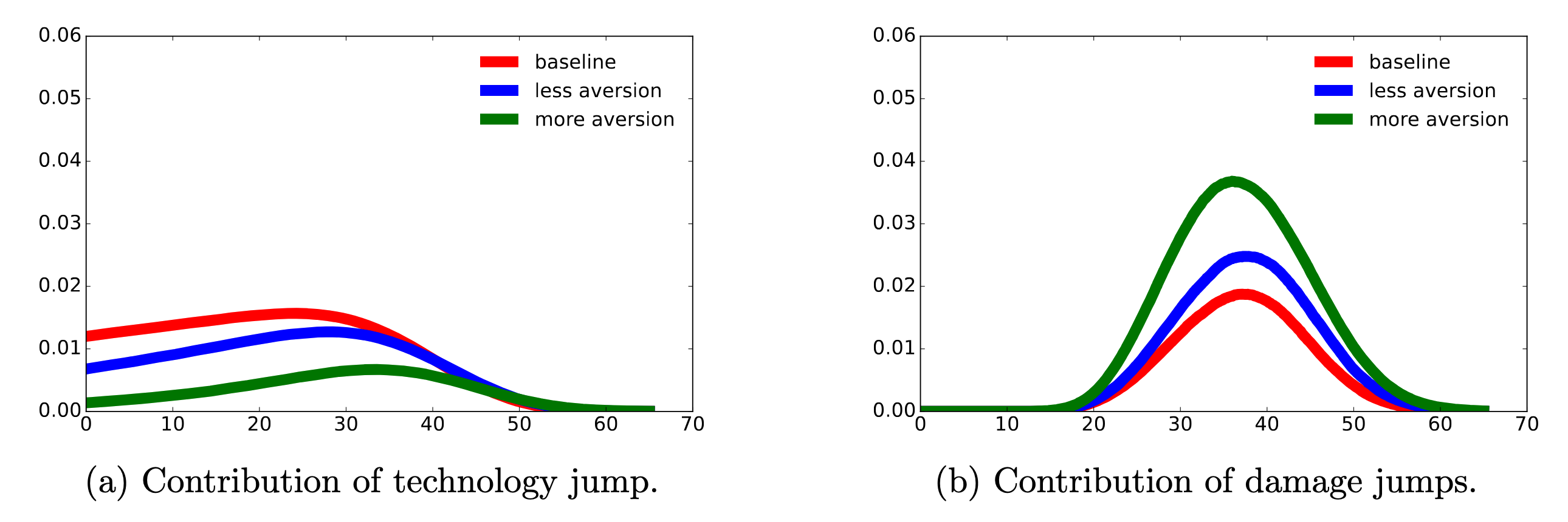
Fig. 11.1 Densities for jump times for different values of \(\xi_m\). For “baseline”, \(\xi_m = \infty\); for “less aversion”, \(\xi_m = .1\); and for “more aversion”, \(\xi_m = .05\). The left plots capture the technology jump-time density contributions when the technology jump happens to occur first; the right plots capture the damage-realization jump-time densities when one of the damage-realization jumps happens to occur first. The integrals of the left densities give the probabilities that the technology jump will happen first, and the integrals of the right densities give the probabilities that a damage-realization jump will happen first.

Fig. 11.2, Fig. 11.3, and Fig. 11.4 give plots based on both Decomposition I and Decomposition II for three different values of \(\xi_m.\) As expected, the expected discounted responses become larger for smaller values of \(\xi_m.\) This due, in part, to the fact that the expectations are computed under the uncertainty-adjusted probability measures. The peak impacts are linked to probabilities that a jump will be realized at the respective horizons. While the R&D knowledge stock prospective responses have the biggest impact on the social value of research and development (SVRD), the capital stock responses are also important. Thus state interactions are a notable aspect of the computations. In contrast, the prospective temperature contributions are very modest and negative. Table 11.2 gives the totals for the SVRD contributions along with the associated investments in the initial time period.

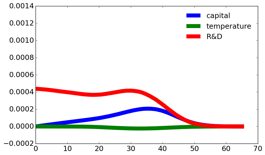
Fig. 11.2 Decompositions of the SVRD are based on time horizon and prospective state variable responses when \(\xi_m = \infty.\) Each flow contribution has been divided by the marginal utility of (damaged) consumption.

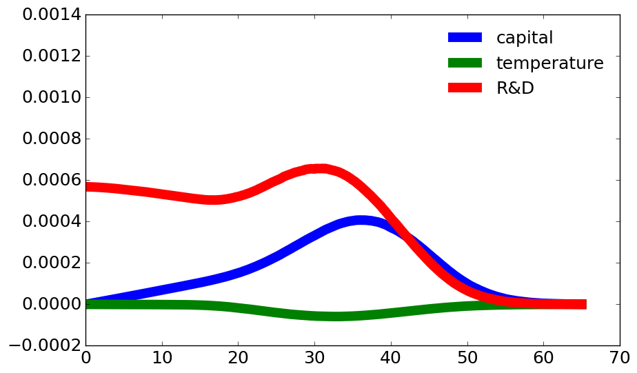
Fig. 11.3 Decompositions of the SVRD are based on time horizon and prospective state variable responses when \(\xi_m = 0.1.\) Each flow contribution has been divided by the marginal utility of (damaged) consumption.

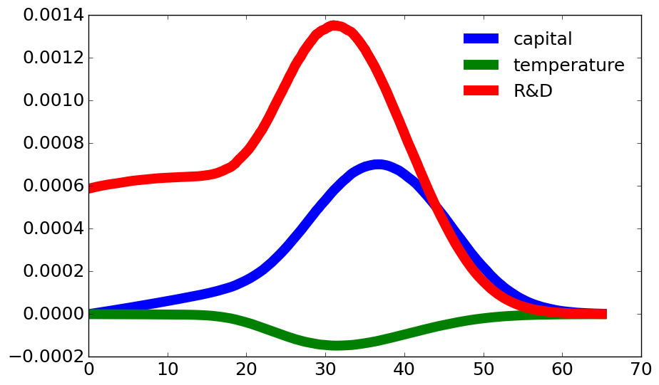
Fig. 11.4 Decompositions of the SVRD’s based on time horizon and prospective state variable responses when \(\xi_m = 0.05.\) Each flow contribution has been divided by the marginal utility of (damaged) consumption.

Table 11.2 Decomposition II of the social value of research and development. Each state contribution has been divided by the marginal utility of (damaged) consumption. Both investments are expressed as a fraction of output.

\(\xi_m\)	capital	temperature	knowledge	sum	R&D investment	capital investment
\(\infty\)	1.15	-0.10	3.50	4.55	.006	.774
.10	2.16	-0.26	5.14	7.04	.014	.766
.05	3.42	-0.63	8.43	11.22	.033	.746

Table 11.3 shows results using Decomposition II for the social cost of global warming (SCGW) along with the emissions in the initial time period. In contrast to the SVRD, the prospective knowledge stock and capital stock contribute to the SCGW in opposite ways. The prospective R&D stock responses decrease the SCGW, as is to be expected. Increased aversion magnifies the SCGW’s. Correspondingly, the emissions are modestly reduced.

Table 11.3 Decomposition II for the SCGW’s. Each state contribution has been divided by the marginal utility of (damaged) consumption.

\(\xi_m\)	capital	temperature	knowledge	sum	emissions
\(\infty\)	14.8	60.4	-15.3	59.9	9.32
.10	37.5	106.0	-40.6	102.9	9.01
.05	84.9	223.0	-94.6	213.3	8.48

Decreasing \(\xi_m\) (increasing robustness concerns) leads to uncertainty-adjusted probabilities that delay the success of R&D. Nevertheless, in the computations so far, Table 11.2 shows an increase in R&D investment for diminished values of \(\xi_m\). It turns out that there is a counteracting force in play that can more than offset the diminished confidence in success prospects. When the robustness concerns are increased, the net success of the discovery, as measured by the continuation value difference \(V^L - V\), becomes larger as the post-jump value function is less exposed to uncertainty. Here the superscript \(L\) denotes the technology success jump. In effect, the endogenously determined payoff to the R&D investment is enhanced. In the results reported so far, this second force dominates. Table 11.4 shows that this is not always true. For a sufficiently small value of \(\xi_m\), say \(\xi_m = .009\), lack of confidence in the investment’s success is sufficient to reverse our previous findings. Thus the R&D investment responses relative to output are not globally monotone in the aversion parameter \(\xi_m.\) In contrast, the SCCC continues to increase and emissions continue to diminish as we reduce \(\xi_m\). We illustrate this outcome in Table 11.5.

Table 11.4 SVRD’s and the R&D investment to output rataio as a function of the robustness parameter, \(\xi_m\).

\(\xi_m\)	SVRD	R&D investment
\(\infty\)	41.3	.006
.10	62.4	.014
.05	95.2	.033
.009	90.0	.031

Table 11.5 SCGW’s and emissions as a function of the robustness parameter, \(\xi_m\).

\(\xi_m\)	SCGW	Emissions
\(\infty\)	54.7	9.32
.10	94.6	9.01
.05	187.3	8.48
.009	677.7	6.26

---

[1]

[Cai et al., 2017]’s measurements are based a planner’s problem that includes explicit risk considerations. [Rennert et al., 2022] use a modular approach to incorporate a wide variety of alternative sources of risk. [Barnett et al., 2025] extends the analysis of [Barnett et al., 2020] use marginal valuation to investigate the uncertainty impacts on the social value of research and development.