Uncertainty Expansion - Computation Process

Author: Haoyang Sun & Faisal Quaiyyum

1 Preliminaries

1.1 Model Setup

\[ \begin{align} X_{t+1} \left( \mathsf{q} \right) = & \hspace{.2cm} \psi^x \left[D_t \left( \mathsf{q} \right), X_{t} \left( \mathsf{q} \right), {\sf q} W_{t+1}, {\sf q} \right], \cr \log G_{t+1} \left( \mathsf{q} \right) - \log G_t \left( \mathsf{q} \right) = & \hspace{.2cm} \psi^g \left[ D_t \left( \mathsf{q} \right), X_{t} \left( \mathsf{q}, \right), {\sf q} W_{t+1}, {\sf q} \right], \cr {\widehat C}_t \left( \mathsf{q} \right) = & \hspace{.2cm} \kappa \left[D_t \left( \mathsf{q} \right), X_{t} \left( \mathsf{q} \right) \right] + {\widehat G}_t \left( \mathsf{q} \right),\cr 0 = & \hspace{.2cm} \phi[D_t({\sf q} ), X_t({\sf q})]. \end{align} \]

In addition, there is a set of first-order conditions and co-state equations detailed in Chapter 10 of the book. Function compile_equations in uncertain_expansion.py pack the state equations, FOC and costate equations for planner’s problem outlined in Appendix 10.A. By default, compile_equations solves the social planner problems. For more general implications, user needs to modify the function compile_equations. The source codes and other dependencies can be found in the src folder of our Github.

1.2 Inputs

The function uncertain_expansion solves models. The function conducts the following steps:

• create_args: initialize the model parameters

• Set up control variables \(D_t\), state variables \(X_t\), growth variables \(\hat G_t\), and static constraints \(\phi\)

• Input an initial guess for \(\left[ {\widehat V_t} - {\widehat C_t}, \widehat C_t - \widehat G_t, D_t, MX_t, MG_t, \widehat G_{t+1} - \widehat G_t, X_t \right]\) in order in initial_guess

• Solve the model using uncertain_expansion

• Plot shock elasticity using plot_exposure_elasticity and plot_price_elasticity

The user must specify several sets of inputs. Define the relevant variables:

Table 1 Variable definitions

Input	Description	Notation in text
control_variables	Variables chosen by the decision-maker at time \(t\)	\(D_t\)
state_variables	Variables that describe the current state of the system	\(X_t\)
shock_variables	Variables representing different entries of the Brownian motion variable	\(W_t\)

The \(t+1\) variables will be automatically created from this. For example, if a state variable is inputted as Z_t, an additional state variable Z_tp1 will be automatically generated. We also need to define the equilibrium conditions:

Table 2 Equation definitions

Input	Description	Notation in text
kappa	Log share of capital not allocated to consumption	\(\kappa(X_t(q),D_t(q))\)
growth	Law of motion for \(\hat{G}_{t+1}-\hat{G}_t\)	\(\psi^g(D_t(q),X_t(q),qW_{t+1},q)\)
state_equations	Law of motion for state variables	\(\psi^x(D_t(q),X_t(q),qW_{t+1},q)\)

The remaining equilibrium conditions will be automatically computed by the code. The user must also define a list of parameters and their corresponding values. This can be done by specifying pairs of inputs such as beta = 0.99 or gamma = 1.01 within the body of the function create_args.

Note that the user must define the variables and parameters before defining the equations. Make sure that the equations use the same expressions for variables and parameters as previously defined by the user.

The output is of class ModelSolution, which stores the coefficients for the linear-quadratic approximation for the jump and state variables; continuation values; consumption growth; and log change of measure, as well as the steady-state values of each variables.

2 Example

We will first solve the internal habit model which is easier to implement as compile_equations compiles FOC and costate equation for social planner problem automatically. Then we will show how to modify compile_equations function to change the FOC condition to external habit model.

We will solve the internal habit model and plot the exposure and price elasticity to replicate figures 10.7-10.10.

import os
import sys
import sympy as sp
workdir = os.getcwd()
# !git clone https://github.com/lphansen/RiskUncertaintyValue 
# workdir = os.getcwd() + '/RiskUncertaintyValue'       
sys.path.insert(0, workdir+'/src')                        
import numpy as np
import seaborn as sns
import autograd.numpy as anp
import matplotlib.pyplot as plt
import pandas as pd
import matplotlib.ticker as mticker 
import matplotlib.cm as cm
from scipy import optimize
np.set_printoptions(suppress=True)
np.set_printoptions(linewidth=200)
from IPython.display import display, HTML
from BY_example_sol import disp_new
display(HTML("<style>.container { width:97% !important; }</style>"))
import warnings
warnings.filterwarnings("ignore")
import matplotlib.pyplot as plt
from scipy.stats import norm

from lin_quad import LinQuadVar
from lin_quad_util import E, concat, next_period, cal_E_ww, lq_sum, N_tilde_measure, E_N_tp1, log_E_exp, kron_prod, distance
from utilities import mat, vec, sym
from uncertain_expansion import uncertain_expansion, generate_symbols_and_args, compile_equations, get_parameter_value, \
    generate_ss_function, automate_step_1, change_parameter_value, approximate_fun ,next_period
from elasticity import exposure_elasticity, price_elasticity
 
np.set_printoptions(suppress=True)
import pickle 
from scipy.optimize import fsolve
# import sympy as sp

2.1 Parameters

Use the function create_args to define and set the parameter values.

def create_args():
    """
    Parameter dictionary for the quarterly calibration (ε = 0.25).
    """
    
    # ---------- Diffusion parameters (Table 1, continuous-time, annual) ----------
    # We store exactly those continuous-time σ's here.
    sigma_k1 = 0.92    * anp.sqrt(12.0)
    sigma_k2 = 0.40    * anp.sqrt(12.0)
    sigma_k3 = 0.0
    sigma_z1 = 0.0
    sigma_z2 = 5.7     * anp.sqrt(12.0)
    sigma_z3 = 0.0
    sigma_y1 = 0.0
    sigma_y2 = 0.0
    sigma_y3 = 0.00031 * anp.sqrt(12.0)
    # ---------- Time step and preferences ----------
    # One model step = one quarter, so ε = 0.25 years.
    epsilon = 0.25                    # Δt in the discretization (years per step)
    delta   = 0.01                    # annual subjective discount rate
    beta    = anp.exp(-delta * epsilon)   # per-quarter discount factor
    # Preferences
    gamma = 1.001
    rho   = 1.001
    # ---------- Technology / adjustment-cost parameters ----------
    a      = 0.0922                # level in log(a - i), unit-free
    # Our equation is: (1/ζ) log(1 + ζ I/K).
    # We encode 1/ζ as phi_1 and ζ as phi_2:
    zeta = 8.0
    phi_1   = 1.0 / zeta               # = 1/ζ
    phi_2   = zeta                     # = ζ
    
    
    # These are *not* time-intensity parameters; they shape the curvature in I/K.
    # ---------- Drifts of state processes (annual, from Table 1) ----------
    alpha_k = 0.04                    # capital drift   (per year)
    beta_k  = 0.04                    # loading of Z_t  (per year)
    beta_z = 0.056                    # Z_t mean reversion (per year)
    beta_2 = 0.194                    # Y_t mean reversion (per year)
    mu_2   = 6.3e-6                   # level in Y_t dynamics (unit-free)
    
    # for habit model
    # nu_h =  0.025 Quarterly habit depreciation rate
    nu_h = 0.1 * epsilon
    tau = 1.01
    llambda = -0.
    return locals()

2.2 Variables

Define your variables as below. You may only have one growth variable and one perturbation variable. Apart from this, you may add more variables to the list as you wish.

Control variable : \(D_t = [\frac{I_{h,t}}{K_t}, \frac{I_{k,t}}{K_t}]'\)

State variable: \(X_t = [Z_{1,t}, Z_{2,t}, X_{1,t}]'\)

Growth variable: \( \hat G_t = \log K_t\)

Perturbation variable: \(q_t\)

Shock Variable: \(W_t = [W_{1,t},W_{2,t},W_{3,t}]\)

# Define variable names
control_variables = ["imh_t", "imk_t"]
state_variables = ["Z_t", "Y_t","X_t"]
growth_variables = ["log_gk_t"]
perturbation_variable = ["q_t"]
shock_variables = ["W1_t", "W2_t", "W3_t"]

The user does not need to change the following code, which creates symbols for the defined parameters and variables.

parameter_names, args = generate_symbols_and_args(create_args)
globals().update(parameter_names)
variables = control_variables + state_variables + growth_variables + perturbation_variable + shock_variables
variables_tp1 = [var + "p1" for var in variables]
symbols = {var: sp.Symbol(var) for var in variables + variables_tp1}
globals().update(symbols)  

2.3 Define Equilibrium Conditions

Ensure that you use the same names for your variables and parameters from before. You must have one output constraint and one capital growth equation, but you may add as many state equations as you wish. The first-order conditions and co-state equations will be automatically handled and do not need to be specified.

State Variable Processes:

\[ \begin{aligned} Z_{1,t+\epsilon} = \hspace{.2cm} & Z_{1,t} - \epsilon \cdot \nu_{1} Z_{1,t} + \sqrt{\epsilon} \cdot \exp\left(\frac 1 2 {Z}_{2,t}\right) \sigma_1 W_{t+1} \cr {Z}_{2,t+\epsilon} = \hspace{.2cm} & {Z}_{2, t} - \epsilon \cdot \nu_2 \left[ 1 - {\mu_2} \exp\left( - {Z}_{2,t} \right) \right] \cr \hspace{.2cm}& - \epsilon \cdot {\frac 1 2} |\sigma_2|^2 \exp\left( - {Z}_{2,t} \right) + \sqrt{\epsilon} \cdot \exp\left( - {\frac 1 2} {Z}_{2,t} \right) \sigma_2 W_{t+1} \cr \log H_{t+\epsilon} - \log K_{t+\epsilon} = \hspace{.2cm} & - \epsilon \cdot \left[ {\frac 1 \zeta} \log \left( 1 + \zeta \frac{I_t}{K_t} \right) - \nu_k Z_{1,t} + \iota_k \right] + \epsilon \cdot \frac{1}{2}|\sigma_k|^2 \exp\left( {Z}_{2,t} \right) - \sqrt{\epsilon} \cdot \exp\left(\frac 1 2 { Z}_{2,t} \right) {\sigma}_k W_{t+\epsilon} \cr & \hspace{.6cm} + \log \left[\exp(-\nu_h + \log H_t - \log K_t) + \left[1 - \exp(-\nu_h)\right] \left(\frac {I_{h,t}}{K_t} \right) \right] \end{aligned}\]

# Technology growth equation
technology_growth = Z_t - epsilon * beta_z * Z_t \
                                + sp.sqrt(epsilon) * sp.exp(0.5 * Y_t) * (sigma_z1 * W1_tp1 + sigma_z2 * W2_tp1 + sigma_z3 * W3_tp1)

# Volatility growth equation
volatility_growth = Y_t - epsilon * beta_2 * (1 - mu_2 * sp.exp(-Y_t)) \
                          - q_t**2 * 0.5 * (sigma_y1**2 + sigma_y2**2 + sigma_y3**2) * sp.exp(-Y_t) * epsilon \
                          + sp.exp(-0.5 * Y_t) * (sigma_y1 * W1_tp1 + sigma_y2 * W2_tp1 + sigma_y3 * W3_tp1) * sp.sqrt(epsilon)


habit_growth = sp.log(sp.exp( - nu_h + X_t) + (1 - sp.exp(-nu_h)) * imh_t ) \
                      - epsilon * (phi_1 * sp.log(1. + phi_2 * imk_t) - alpha_k + beta_k * Z_t \
                      - q_t**2 * 0.5 * (sigma_k1**2 + sigma_k2**2 + sigma_k3**2) * sp.exp(Y_t)) \
                      - sp.sqrt(epsilon) * sp.exp(0.5 * Y_t) * (sigma_k1 * W1_tp1 + sigma_k2 * W2_tp1 + sigma_k3 * W3_tp1) 

Growth Process:

\[\begin{split} \begin{aligned} \widehat K_{t+\epsilon } - \widehat K_t = & \epsilon \cdot \left[\frac{1}{\zeta}\log\!\left(1+\zeta\frac{I_t}{K_t}\right) + \nu_k Z_{1,t} - \iota_k \right] \\ & - \frac12 |\sigma_k|^2 e^{Z_{2,t}} + \sqrt{\epsilon} \cdot e^{\frac12 Z_{2,t}} \sigma_k W_{t+\epsilon} \end{aligned} \end{split}\]

# Capital growth equation
capital_growth = epsilon * (phi_1 * sp.log(1. + phi_2 * imk_t) - alpha_k + beta_k * Z_t \
                      - q_t**2 * 0.5 * (sigma_k1**2 + sigma_k2**2 + sigma_k3**2) * sp.exp(Y_t)) \
                      + sp.sqrt(epsilon) * sp.exp(0.5 * Y_t) * (sigma_k1 * W1_tp1 + sigma_k2 * W2_tp1 + sigma_k3 * W3_tp1) 

Output constraint: $\({\hat C}_t - \hat G_{t}=\kappa(D_t, X_t) = \frac{1}{1 - \tau} \log( (1 - \lambda) D^{1 - \tau} + \lambda \exp((1 - \tau) X) )\)$

# Output constraint
kappa = 1/(1 - tau) *  sp.log( (1 - llambda) * imh_t**(1 - tau) + llambda * sp.exp((1 - tau) * X_t ))

The static constraint: \(0 = \alpha - \frac{I_{h,t}}{K_t} - \frac{I_{k,t}}{K_t}\)

# static constraints
phi1 =   a -imh_t - imk_t  

output_constraint = kappa 
static_constraints = [phi1]
state_equations = [technology_growth, volatility_growth,habit_growth]

2.4 Code Settings

You may additionally set the following:

• Initial guess for steady-state variables. This must have the same length as the number of variables

• Convergence tolerance. How small the maximum error across the approximated terms must be before the algorithm is considered to have converged.

• Maximum iterations. The maximum number of iterations for the algorithm can take.

• Save location. Save the model solution to this location so that it can be accessed later.

The order of the initial guess is as follows:

\[ \left[ {\widehat V_t} - {\widehat C_t}, \widehat C_t - \widehat G_t, D_t, MX_t, MG_t, \widehat G_{t+1} - \widehat G_t, X_t \right] \]

initial_guess = np.array([ -3.0599204508041717, -3.1433984583550463, (1 - anp.exp(-0.01 * 0.25)) / 0.0257233 , 0.0257233 , 0.0922 - 0.0257233,  0.02039991,   0.        ,   0.2        ,  \
                           1.        ,   0.01330655,   0.        , -11.97496092,  -3.51858229])

savepath = None
init_util = None
iter_tol = 1e-5
max_iter = 500 

2.5 Run Code

You are now ready to run the function uncertain_expansion. You do not need to change anything in the following code.

ModelSol = uncertain_expansion(control_variables, state_variables, shock_variables, variables, variables_tp1,
                            kappa, capital_growth, state_equations, static_constraints, initial_guess, parameter_names,
                            args, approach = '1', init_util = init_util, iter_tol = iter_tol, max_iter = max_iter,
                            savepath=savepath)
ModelSol.ss

Show code cell output Hide code cell output

Iteration 1: mu_0 error = 3.04931861e-19
Iteration 1: J1 error = 0.000561672114
Iteration 1: J2 error = 0.000554623791
Iteration 1: error = 0.000561672114
The iteration is not making good progress, as measured by the 
  improvement from the last ten iterations.
Iteration 2: mu_0 error = 5.08219768e-20
Iteration 2: J1 error = 8.52838789e-08
Iteration 2: J2 error = 7.83537071e-08
Iteration 2: error = 8.52838789e-08

array([ -4.12667104,   0.15503472,   0.01613651,   0.07606349,   0.60576715,   0.        ,  -0.        ,   1.        ,   0.00485334,  -0.        , -11.97496092,  -4.30652983])

In the homework, you are asked to solve the models with different parameters and compare the results. Here we give an example to loops over \(\gamma\) and \(\lambda\) and saves them to appropriately.

Good initial guesses are important for solving the model successfully. Models with negative \(\lambda\) are easier to solve. We use the trick that solving easier model first, and use the solution as initial guess for models with larger \(\lambda\). We stored the solved model in the folder output.

gamma_values  = [1.001, 4.0, 8.0]
lambda_values = [-9.0, -5.0, -4.0,-3.0,-2.0 ,-1.0,0.0, 0.1, 0.2, 0.3, 0.4,0.5,0.6, 0.7, 0.8, 0.9] 

initial_guess_baseline = initial_guess.copy()  
preloadpath = None  

for gamma_i in gamma_values:
    # update gamma once per outer loop
    args = change_parameter_value('gamma', parameter_names, args, gamma_i)
    print(f"gamma: {gamma_i}")

    # store the last solution’s steady state for this gamma
    prev_ss = None

    for llambda_i in lambda_values:
        llambda_i = round(llambda_i, 2)
        args = change_parameter_value('llambda', parameter_names, args, llambda_i)
        print(f"lambda: {llambda_i}")

        savepath = f'output/res_gamma_{gamma_i}_lambda_{llambda_i}.pkl'

        # 0. If this parameter combo was already solved before, just load & move on
        if os.path.exists(savepath):
            with open(savepath, 'rb') as f:
                res = pickle.load(f)
            prev_ss = res['ss']
            print("  -> loaded existing solution from disk")
            continue

        # 1. Choose initial_guess:
        if prev_ss is not None:
            # use solution from previous λ for this γ
            initial_guess = np.concatenate([np.array([-3.40379947]), prev_ss])
        elif preloadpath is not None and os.path.exists(preloadpath):
            # optional: use some external “easy” case as a starting point
            with open(preloadpath, 'rb') as f:
                preload = pickle.load(f)
            initial_guess = np.concatenate([np.array([-3.40379947]), preload['ss']])
        else:
            # fall back to your original global guess
            initial_guess = initial_guess_baseline

        # 2. Solve at (gamma_i, llambda_i)
        res = uncertain_expansion(
            control_variables, state_variables, shock_variables,
            variables, variables_tp1,
            kappa, capital_growth, state_equations, static_constraints,
            initial_guess, parameter_names,
            args, approach='1', init_util=init_util,
            iter_tol=iter_tol, max_iter=max_iter,
            savepath=savepath,   # still writes to disk inside
        )

        # 3. Store this steady state to warm-start the next λ
        prev_ss = res['ss']

        # and optionally make this the preload for future runs / sessions
        preloadpath = savepath

# Grids
gamma_values  = [1.001, 4.0, 8.0] 
# 0.5-step grid from 0 down to -9
# lambda_values =  [round(l, 1) for l in np.arange(0.0, -0.8, -0.1)] 
lambda_values = [ -1.0]
# lambda_values = [round(l, 2) for l in np.arange(-0.7, -1.0, -0.01)] 
# lambda_values = [   -4, -6]
tau_fixed     = 1.001
# tau_fixed     = 0.01

initial_guess_baseline = initial_guess.copy()
preloadpath = None

for gamma_i in gamma_values:
    args = change_parameter_value('gamma', parameter_names, args, gamma_i)
    print(f"gamma: {gamma_i}")

    # fix tau = 2.0
    args = change_parameter_value('tau', parameter_names, args, tau_fixed)
    print(f"  tau: {tau_fixed}")

    prev_ss_lambda = None  # warm-start across lambda at tau=2.0 for this gamma

    for llambda_i in lambda_values:
        llambda_i = float(llambda_i)
        args = change_parameter_value('llambda', parameter_names, args, llambda_i)
        print(f"    lambda: {llambda_i}")

        tau_str    = f"{tau_fixed:.2f}"
        lambda_str = f"{llambda_i:.2f}"

        # file for this (gamma, lambda, tau=2.0)
        savepath = f'output/res_gamma_{gamma_i}_lambda_{lambda_str}_tau_{tau_str}.pkl'

        # 0. If already solved, load and move on
        if os.path.exists(savepath):
            with open(savepath, 'rb') as f:
                res = pickle.load(f)
            prev_ss_lambda = res['ss']
            print("      -> loaded existing (gamma, lambda, tau=2.0) solution from disk")
            continue

        # 1. initial_guess hierarchy (NO tau=1.01 baseline)
        if prev_ss_lambda is not None:
            # previous lambda at tau=2.0 for this gamma
            initial_guess = np.concatenate([np.array([-10.40379947]), prev_ss_lambda])
        elif preloadpath is not None and os.path.exists(preloadpath):
            # last solved parameter combo (any gamma, lambda)
            with open(preloadpath, 'rb') as f:
                preload = pickle.load(f)
            initial_guess = np.concatenate([np.array([-10.40379947]), preload['ss']])
        else:
            # global fallback
            initial_guess = initial_guess_baseline

        # 2. Solve at (gamma_i, llambda_i, tau_fixed)
        res = uncertain_expansion(
            control_variables, state_variables, shock_variables,
            variables, variables_tp1,
            kappa, capital_growth, state_equations, static_constraints,
            initial_guess, parameter_names,
            args, approach='2', init_util=init_util,
            iter_tol=iter_tol, max_iter=max_iter,
            savepath=savepath,
        )
    
        # 3. warm-start next lambda and remember last solved solution
        prev_ss_lambda = res['ss']
        preloadpath = savepath

gamma: 1.001
  tau: 1.001
    lambda: -1.0
      -> loaded existing (gamma, lambda, tau=2.0) solution from disk
gamma: 4.0
  tau: 1.001
    lambda: -1.0
      -> loaded existing (gamma, lambda, tau=2.0) solution from disk
gamma: 8.0
  tau: 1.001
    lambda: -1.0
The iteration is not making good progress, as measured by the 
  improvement from the last ten iterations.
Iteration 1: mu_0 error = 9.15933995e-16
Iteration 1: J1 error = 0.0236735392
Iteration 1: J2 error = 0.0490929176
Iteration 1: error = 0.0490929176
Iteration 2: mu_0 error = 2.22044605e-16
Iteration 2: J1 error = 2.65994357e-05
Iteration 2: J2 error = 5.99795346e-06
Iteration 2: error = 2.65994357e-05
Iteration 3: mu_0 error = 1.11022302e-15
Iteration 3: J1 error = 3.68514702e-08
Iteration 3: J2 error = 1.11329649e-08
Iteration 3: error = 3.68514702e-08

# Figure 10.5 with different tau
# Solve models
# Grids
gamma_values  = [1.001, 4.0, 8.0] 
# lambda_values = [0.9, 0.0, -0.9]
lambda_values = [ -1.0]
# tau: [1.01, 0.9, 0.8, ..., 0.2]
# tau_values = [1.001, 0.9, 0.8,0.7,0.6,0.5,0.4, 0.3, 0.2, 0.15, 0.1, 0.05, 0.01, 0.0, -0.1, -0.2, -0.3, -0.4, -0.5, -0.6, -0.7 ]
tau_values = [1.001, 0.6,0.01  ]

initial_guess_baseline = initial_guess.copy()

# "use the last solution as next initial guess" (across ALL (lambda, tau) combos)
prev_ss_last = None

for gamma_i in gamma_values:
    args = change_parameter_value('gamma', parameter_names, args, gamma_i)
    print(f"gamma: {gamma_i}")

    for llambda_i in lambda_values:
        llambda_i = float(llambda_i)
        args = change_parameter_value('llambda', parameter_names, args, llambda_i)
        print(f"  lambda: {llambda_i}")

        for tau_i in tau_values:
            tau_i = float(tau_i)
            args = change_parameter_value('tau', parameter_names, args, tau_i)
            print(f"    tau: {tau_i}")

            tau_str    = f"{tau_i:.3f}"
            lambda_str = f"{llambda_i:.1f}"

            savepath = f"output/res_gamma_{gamma_i}_lambda_{lambda_str}_tau_{tau_str}.pkl"

            # 0) If already solved, load it and use as the next initial guess
            if os.path.exists(savepath):
                with open(savepath, "rb") as f:
                    res = pickle.load(f)
                prev_ss_last = res["ss"]
                print("      -> loaded existing solution from disk (warm-start updated)")
                continue

            # 1) Initial guess: always warm-start from the most recently solved combo if available
            if prev_ss_last is not None:
                initial_guess = np.concatenate([np.array([-10.40379947]), prev_ss_last])
            else:
                initial_guess = initial_guess_baseline

            # 2) Solve at (gamma_i, llambda_i, tau_i)
            res = uncertain_expansion(
                control_variables, state_variables, shock_variables,
                variables, variables_tp1,
                kappa, capital_growth, state_equations, static_constraints,
                initial_guess, parameter_names,
                args, approach="2", init_util=init_util,
                iter_tol=iter_tol, max_iter=max_iter,
                savepath=savepath,
            )

            # 3) Warm-start the next point
            prev_ss_last = res["ss"]

gamma: 1.001
  lambda: -1.0
    tau: 1.001
Iteration 1: mu_0 error = 2.6427428e-19
Iteration 1: J1 error = 0.000919146607
Iteration 1: J2 error = 0.000940954302
Iteration 1: error = 0.000940954302
Iteration 2: mu_0 error = 1.82959117e-19
Iteration 2: J1 error = 2.23369241e-07
Iteration 2: J2 error = 2.21425295e-07
Iteration 2: error = 2.23369241e-07
    tau: 0.6
Iteration 1: mu_0 error = 2.74438675e-19
Iteration 1: J1 error = 0.000695657395
Iteration 1: J2 error = 0.000789904985
Iteration 1: error = 0.000789904985
Iteration 2: mu_0 error = 1.93123512e-19
Iteration 2: J1 error = 1.2998525e-07
Iteration 2: J2 error = 1.50145667e-07
Iteration 2: error = 1.50145667e-07
    tau: 0.01
Iteration 1: mu_0 error = 1.42301535e-19
Iteration 1: J1 error = 0.000544146216
Iteration 1: J2 error = 0.000511294666
Iteration 1: error = 0.000544146216
Iteration 2: mu_0 error = 4.7433845e-20
Iteration 2: J1 error = 8.31676037e-08
Iteration 2: J2 error = 7.78133107e-08
Iteration 2: error = 8.31676037e-08
gamma: 4.0
  lambda: -1.0
    tau: 1.001
Iteration 1: mu_0 error = 3.46944695e-17
Iteration 1: J1 error = 0.0101458025
Iteration 1: J2 error = 0.0209661763
Iteration 1: error = 0.0209661763
Iteration 2: mu_0 error = 4.51028104e-16
Iteration 2: J1 error = 1.12699286e-05
Iteration 2: J2 error = 1.41537142e-06
Iteration 2: error = 1.12699286e-05
Iteration 3: mu_0 error = 3.1918912e-16
Iteration 3: J1 error = 1.57617441e-08
Iteration 3: J2 error = 3.1926457e-09
Iteration 3: error = 1.57617441e-08
    tau: 0.6
Iteration 1: mu_0 error = 5.41233725e-16
Iteration 1: J1 error = 0.00997359781
Iteration 1: J2 error = 0.0207076969
Iteration 1: error = 0.0207076969
Iteration 2: mu_0 error = 2.01227923e-16
Iteration 2: J1 error = 1.20182962e-05
Iteration 2: J2 error = 3.02414754e-06
Iteration 2: error = 1.20182962e-05
Iteration 3: mu_0 error = 6.17561557e-16
Iteration 3: J1 error = 1.37463582e-08
Iteration 3: J2 error = 4.74746475e-09
Iteration 3: error = 1.37463582e-08
    tau: 0.01
Iteration 1: mu_0 error = 4.16333634e-17
Iteration 1: J1 error = 0.0110164038
Iteration 1: J2 error = 0.0203704283
Iteration 1: error = 0.0203704283
Iteration 2: mu_0 error = 4.37150316e-16
Iteration 2: J1 error = 1.15368617e-05
Iteration 2: J2 error = 1.0236902e-06
Iteration 2: error = 1.15368617e-05
Iteration 3: mu_0 error = 4.64905892e-16
Iteration 3: J1 error = 1.10811155e-08
Iteration 3: J2 error = 2.0238039e-09
Iteration 3: error = 1.10811155e-08
gamma: 8.0
  lambda: -1.0
    tau: 1.001
Iteration 1: mu_0 error = 2.63677968e-15
Iteration 1: J1 error = 0.0236735392
Iteration 1: J2 error = 0.0490929176
Iteration 1: error = 0.0490929176
Iteration 2: mu_0 error = 2.19269047e-15
Iteration 2: J1 error = 2.65994357e-05
Iteration 2: J2 error = 5.99795348e-06
Iteration 2: error = 2.65994357e-05
Iteration 3: mu_0 error = 1.11022302e-15
Iteration 3: J1 error = 3.68514773e-08
Iteration 3: J2 error = 1.11329699e-08
Iteration 3: error = 3.68514773e-08
    tau: 0.6
Iteration 1: mu_0 error = 8.60422844e-16
Iteration 1: J1 error = 0.0242040149
Iteration 1: J2 error = 0.0485869979
Iteration 1: error = 0.0485869979
Iteration 2: mu_0 error = 9.15933995e-16
Iteration 2: J1 error = 2.8221406e-05
Iteration 2: J2 error = 1.1982034e-05
Iteration 2: error = 2.8221406e-05
Iteration 3: mu_0 error = 1.16573418e-15
Iteration 3: J1 error = 3.21088444e-08
Iteration 3: J2 error = 1.74065756e-08
Iteration 3: error = 3.21088444e-08
    tau: 0.01
Iteration 1: mu_0 error = 3.60822483e-16
Iteration 1: J1 error = 0.0264356103
Iteration 1: J2 error = 0.047875198
Iteration 1: error = 0.047875198
Iteration 2: mu_0 error = 5.13478149e-16
Iteration 2: J1 error = 2.70354003e-05
Iteration 2: J2 error = 8.85365581e-06
Iteration 2: error = 2.70354003e-05
Iteration 3: mu_0 error = 1.52655666e-15
Iteration 3: J1 error = 2.58735113e-08
Iteration 3: J2 error = 1.1831286e-08
Iteration 3: error = 2.58735113e-08

# Grids
gamma_values  = [1.001, 4.0, 8.0] 
# 0.5-step grid from 0 down to -9
lambda_values = [-0.7] 
# lambda_values = [   -4, -6]
tau_fixed     = 2.0
stored_models ={}
initial_guess_baseline = initial_guess.copy()
preloadpath = None

for gamma_i in gamma_values:
    args = change_parameter_value('gamma', parameter_names, args, gamma_i)
    print(f"gamma: {gamma_i}")

    # fix tau = 2.0
    args = change_parameter_value('tau', parameter_names, args, tau_fixed)
    print(f"  tau: {tau_fixed}")

    prev_ss_lambda = None  # warm-start across lambda at tau=2.0 for this gamma

    for llambda_i in lambda_values:
        llambda_i = float(llambda_i)
        args = change_parameter_value('llambda', parameter_names, args, llambda_i)
        print(f"    lambda: {llambda_i}")

        tau_str    = f"{tau_fixed:.2f}"
        lambda_str = f"{llambda_i:.1f}"

        # file for this (gamma, lambda, tau=2.0)
        savepath = f'output/res_gamma_{gamma_i}_lambda_{lambda_str}_tau_{tau_str}.pkl'
 
        # 1. initial_guess hierarchy (NO tau=1.01 baseline)
        if prev_ss_lambda is not None:
            # previous lambda at tau=2.0 for this gamma
            initial_guess = np.concatenate([np.array([-10.40379947]), prev_ss_lambda])
        elif preloadpath is not None and os.path.exists(preloadpath):
            # last solved parameter combo (any gamma, lambda)
            with open(preloadpath, 'rb') as f:
                preload = pickle.load(f)
            initial_guess = np.concatenate([np.array([-10.40379947]), preload['ss']])
        else:
            # global fallback
            initial_guess = initial_guess_baseline

        # 2. Solve at (gamma_i, llambda_i, tau_fixed)
        res = uncertain_expansion(
            control_variables, state_variables, shock_variables,
            variables, variables_tp1,
            kappa, capital_growth, state_equations, static_constraints,
            initial_guess, parameter_names,
            args, approach='2', init_util=init_util,
            iter_tol=iter_tol, max_iter=max_iter,
            savepath=savepath,
        )
        stored_models[gamma_i] = res
    
        # 3. warm-start next lambda and remember last solved solution
        prev_ss_lambda = res['ss']
        preloadpath = savepath

gamma: 1.001
  tau: 2.0
    lambda: -0.7
Iteration 1: mu_0 error = 1.34847645e-18
Iteration 1: J1 error = 0.00824409812
Iteration 1: J2 error = 2.30317556
Iteration 1: error = 2.30317556
Iteration 2: mu_0 error = 4.50621528e-19
Iteration 2: J1 error = 1.15287213e-05
Iteration 2: J2 error = 0.00398208257
Iteration 2: error = 0.00398208257
Iteration 3: mu_0 error = 1.28749008e-19
Iteration 3: J1 error = 1.8149322e-08
Iteration 3: J2 error = 6.35118317e-06
Iteration 3: error = 6.35118317e-06
gamma: 4.0
  tau: 2.0
    lambda: -0.7
Iteration 1: mu_0 error = 9.36750677e-16
Iteration 1: J1 error = 0.0473814511
Iteration 1: J2 error = 11.8012178
Iteration 1: error = 11.8012178
Iteration 2: mu_0 error = 4.37150316e-16
Iteration 2: J1 error = 0.000272087818
Iteration 2: J2 error = 0.0745181164
Iteration 2: error = 0.0745181164
Iteration 3: mu_0 error = 2.09554596e-15
Iteration 3: J1 error = 1.76813302e-06
Iteration 3: J2 error = 0.000484779568
Iteration 3: error = 0.000484779568
Iteration 4: mu_0 error = 2.59514632e-15
Iteration 4: J1 error = 1.18110304e-08
Iteration 4: J2 error = 3.24811117e-06
Iteration 4: error = 3.24811117e-06
gamma: 8.0
  tau: 2.0
    lambda: -0.7
Iteration 1: mu_0 error = 4.19109192e-15
Iteration 1: J1 error = 0.0995819886
Iteration 1: J2 error = 24.4044909
Iteration 1: error = 24.4044909
Iteration 2: mu_0 error = 4.16333634e-16
Iteration 2: J1 error = 0.000619615789
Iteration 2: J2 error = 0.168974351
Iteration 2: error = 0.168974351
Iteration 3: mu_0 error = 5.91193761e-15
Iteration 3: J1 error = 4.10222269e-06
Iteration 3: J2 error = 0.00113400246
Iteration 3: error = 0.00113400246
Iteration 4: mu_0 error = 2.88657986e-15
Iteration 4: J1 error = 2.75212422e-08
Iteration 4: J2 error = 7.70379779e-06
Iteration 4: error = 7.70379779e-06

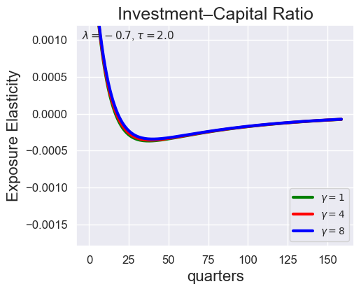
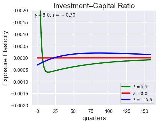
# Investment-Capital Ratio Elasticity with negative Tau

import numpy as np
import sympy as sp
import matplotlib.pyplot as plt
import seaborn as sns

def plot_growth_shock_investment_gamma_only(models_dict, T, ylim_i=None, save_path=None,
                                           llambda=-0.7, tau=2.0):
    """
    Exposure Elasticity for GROWTH SHOCK only.
    Single figure: Investment-Capital Ratio (for gamma = 1.001, 4.001, 8.001) at fixed lambda, tau.
    """
    sns.set_style("darkgrid")

    gammas_ordered = [1.001, 4.0, 8.0]
    colors = ['green', 'red', 'blue']
    labels = [r'$\gamma=1$', r'$\gamma=4$', r'$\gamma=8$']

    fig, ax = plt.subplots(1, 1, figsize=(5.5, 4.5))
    time_axis = np.arange(T)

    imk_t_sym = sp.Symbol('imk_t')
    target_expression = sp.log(imk_t_sym)

    for idx, g in enumerate(gammas_ordered):
        if g not in models_dict:
            print(f"Warning: Model for gamma={g} not found.")
            continue

        mod = models_dict[g]

        # dict-like access (ModelSolution) should work with []
        log_IK_t, _, _, _ = approximate_fun(
            fun=target_expression,
            ss=mod["ss"],
            ss_variables=mod["ss_variables"],
            ss_variables_tp1=mod["ss_variables_tp1"],
            parameter_names=mod["parameter_names"],
            args=mod["args"],
            var_shape=mod["var_shape"],
            JX1_t=mod["JX1_t"],
            JX2_t=mod["JX2_t"],
            X1_tp1=mod["X1_tp1"],
            X2_tp1=mod["X2_tp1"],
            recursive_ss=mod["recursive_ss"],
            second_order=True
        )

        log_IK_tp1 = next_period(log_IK_t, mod["X1_tp1"], mod["X2_tp1"])
        log_IK_growth = log_IK_tp1 - log_IK_t

        elas_i = exposure_elasticity(
            log_IK_growth, mod["X1_tp1"], mod["X2_tp1"], T, shock=1, percentile=0.5
        ).flatten()

        sns.lineplot(x=time_axis, y=elas_i, ax=ax, color=colors[idx], label=labels[idx], linewidth=3.0)

    ax.set_title("Investment–Capital Ratio", fontsize=18)
    ax.set_ylabel(r"Exposure Elasticity", fontsize=16)
    ax.set_xlabel("quarters", fontsize=16)
    ax.tick_params(axis="both", labelsize=12)
    ax.legend(fontsize=10, loc="lower right")

    ax.text(0.02, 0.98, rf"$\lambda={llambda}$, $\tau={tau}$",
            transform=ax.transAxes, va="top", ha="left", fontsize=11)

    if ylim_i is not None:
        ax.set_ylim(ylim_i)
    else:
        ax.set_ylim(bottom=0)

    plt.tight_layout()
    if save_path is not None:
        plt.savefig(save_path, dpi=300, bbox_inches="tight")
    plt.show()


plot_growth_shock_investment_gamma_only(
    stored_models,
    T=160,
    ylim_i=[-0.0018, 0.0012],
    llambda=-0.7,
    tau=2.0
)

import os, pickle
import numpy as np
import sympy as sp
import matplotlib.pyplot as plt
import seaborn as sns

def load_models_for_tau_three_lambdas(
    tau,
    lambdas=(0.9, 0.0, -9.0),
    gamma=8.0,
    output_dir="output",
):
    """
    Load models for a fixed (gamma, tau) across multiple lambdas.
    Returns: dict keyed by lambda -> loaded model dict (the pickle content).
    """
    models_by_lambda = {}

    tau_str = f"{float(tau):.2f}"
    for lam in lambdas:
        lam = float(lam)
        lam_str = f"{lam:.1f}"
        path = os.path.join(output_dir, f"res_gamma_{gamma}_lambda_{lam_str}_tau_{tau_str}.pkl")

        if not os.path.exists(path):
            print(f"[load warning] missing: {path}")
            continue

        with open(path, "rb") as f:
            models_by_lambda[lam] = pickle.load(f)

    return models_by_lambda


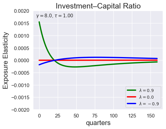
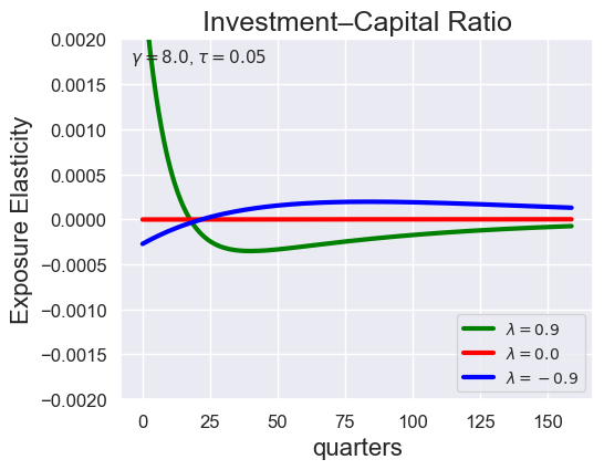
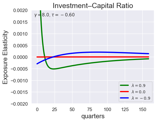
def plot_growth_shock_investment_lambda_only(
    models_by_lambda,
    T,
    tau,
    lambdas=(0.9, 0.0, -9.0),
    gamma=8.0,
    ylim_i=(-2e-3, 2e-3),
    save_path=None,
    shock=1,
    percentile=0.5,
):
    """
    Exposure Elasticity for GROWTH SHOCK only.
    Single figure: Investment–Capital Ratio elasticity for 3 lambdas at fixed (gamma, tau).
    """
    sns.set_style("darkgrid")

    lambdas_ordered = [float(x) for x in lambdas]
    colors = ["green", "red", "blue"]
    labels = [rf"$\lambda={l:.1f}$" for l in lambdas_ordered]

    fig, ax = plt.subplots(1, 1, figsize=(5.8, 4.6))
    time_axis = np.arange(T)

    imk_t_sym = sp.Symbol("imk_t")
    target_expression = sp.log(imk_t_sym)

    for idx, lam in enumerate(lambdas_ordered):
        if lam not in models_by_lambda:
            print(f"[plot warning] model not found for lambda={lam}")
            continue

        mod = models_by_lambda[lam]

        log_IK_t, _, _, _ = approximate_fun(
            fun=target_expression,
            ss=mod["ss"],
            ss_variables=mod["ss_variables"],
            ss_variables_tp1=mod["ss_variables_tp1"],
            parameter_names=mod["parameter_names"],
            args=mod["args"],
            var_shape=mod["var_shape"],
            JX1_t=mod["JX1_t"],
            JX2_t=mod["JX2_t"],
            X1_tp1=mod["X1_tp1"],
            X2_tp1=mod["X2_tp1"],
            recursive_ss=mod["recursive_ss"],
            second_order=True,
        )

        log_IK_tp1 = next_period(log_IK_t, mod["X1_tp1"], mod["X2_tp1"])
        log_IK_growth = log_IK_tp1 - log_IK_t

        elas = exposure_elasticity(
            log_IK_growth, mod["X1_tp1"], mod["X2_tp1"],
            T, shock=shock, percentile=percentile
        ).flatten()

        sns.lineplot(
            x=time_axis, y=elas, ax=ax,
            color=colors[idx % len(colors)],
            label=labels[idx],
            linewidth=3.0,
        )

    ax.set_title("Investment–Capital Ratio", fontsize=18)
    ax.set_ylabel("Exposure Elasticity", fontsize=16)
    ax.set_xlabel("quarters", fontsize=16)
    ax.tick_params(axis="both", labelsize=12)
    ax.legend(fontsize=10, loc="lower right")

    ax.text(
        0.02, 0.98,
        rf"$\gamma={gamma}$, $\tau={float(tau):.2f}$",
        transform=ax.transAxes, va="top", ha="left", fontsize=11
    )

    if ylim_i is not None:
        ax.set_ylim(ylim_i)

    plt.tight_layout()
    if save_path is not None:
        plt.savefig(save_path, dpi=300, bbox_inches="tight")
    plt.show()
tau_values = [ 1.001,   0.8, 0.6, 0.4,   0.2,   0.1, 0.05,  0.0, -0.1, -0.2, -0.3, -0.4, -0.5, -0.6, -0.7 ]
lambdas = (0.9, 0.0, -0.9)

for tau in tau_values:
    models_tau = load_models_for_tau_three_lambdas(tau=tau, lambdas=lambdas, gamma=8.0)
    plot_growth_shock_investment_lambda_only(models_tau, T=160, tau=tau, lambdas=lambdas, gamma=8.0)

Note that the order of the variables listed in the solution is the same as before, except with \({\widehat V_t} - {\widehat C_t}\) removed:

\[ \left[ \widehat C_t - \widehat K_t, D_t, MX_t, MG_t, \widehat G_{t+1} - \widehat G_t, X_t \right] \]

2.6 Plot Elasticities

After you used the loop above, you can also use the following code to load all your solutions dynamically:

models = {}
gamma_values = [1.001, 4.001,  8.001] 
lambda_values = [-9.0,   0.0,  0.9]
for gamma_i in gamma_values:
    for llambda_i in lambda_values:
        llambda_i = round(llambda_i,2)
        save_path = 'output/res_gamma_{}_lambda_{}.pkl'.format(gamma_i, llambda_i)
        try:
            with open(save_path, 'rb') as f:
                # models = pickle.load(save_path)
                model_key = f"gamma_{gamma_i}_lambda_{llambda_i}"
                models[model_key] = pickle.load(f)
        except FileNotFoundError:
            print(f"File not found: {save_path}")

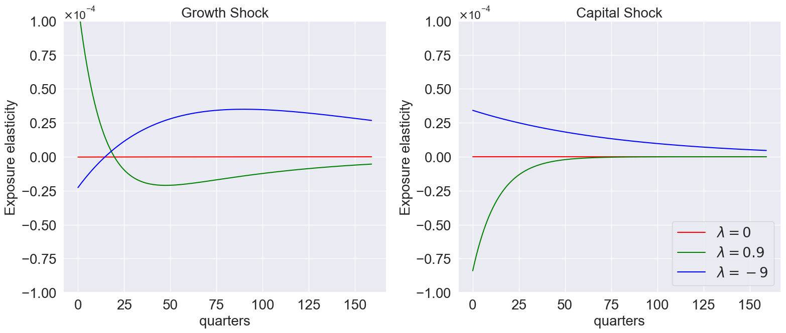
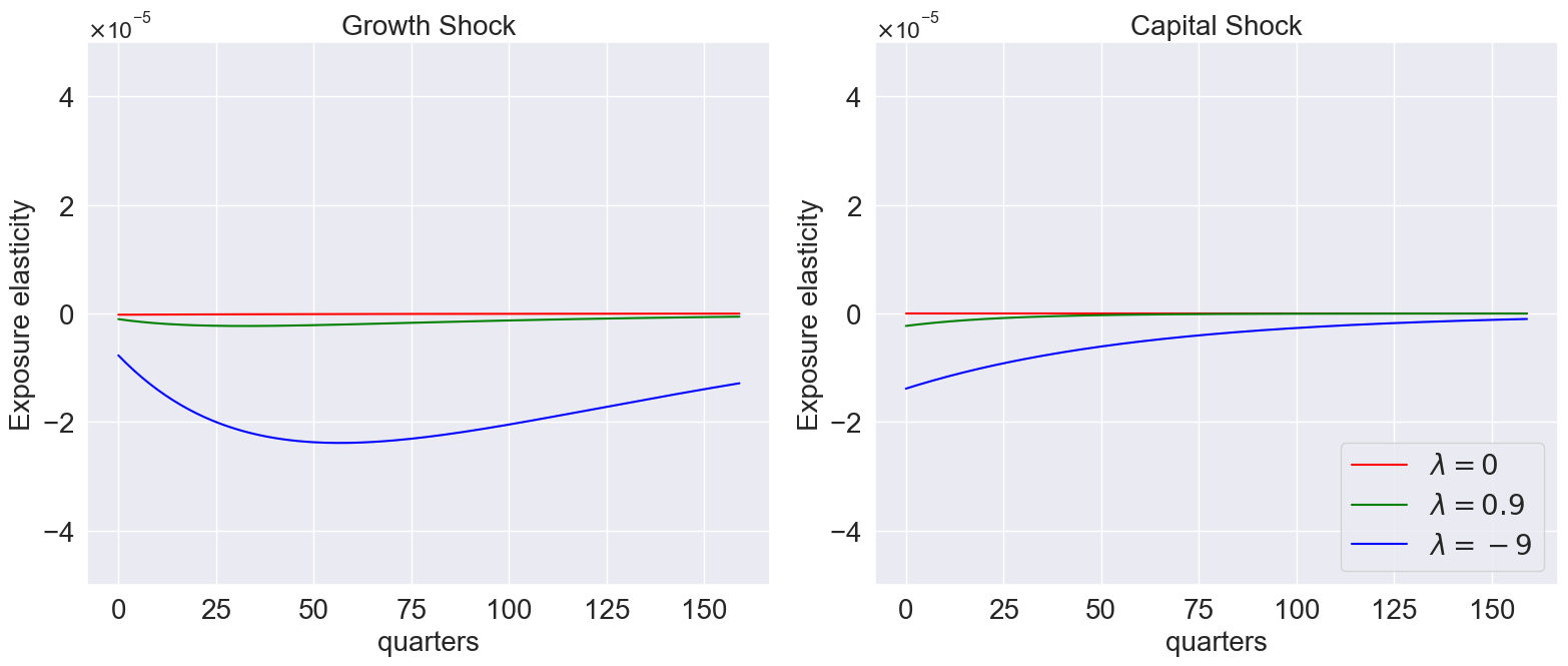
We can use plot_exposure_elasticity_shocks to plot exposure elasticities for different shocks.

• model_list is a list of solutions you want to use to compute elasticities

• logMtM0 specifies the quantity for which you are calculating the elasticity

• T specifies the number of periods (using the time-unit that you specified the parameters in)

• num_shocks specifies the number of shocks to calculate

def plot_exposure_elasticity_shocks(
    model_list, 
    Mtgrowth_list,
    quantile, 
    T, 
    num_shocks, 
    time_unit='quarters', 
    ylimits=None, 
    labels=None, 
    title=None, 
    shock_names=None, 
    colors=None, 
    save_path=None
):
    """
    Plot exposure elasticity for multiple models across different shocks.
    
    Parameters:
    - model_list: List of model results to plot.
    - quantile: List of quantiles to calculate.
    - T: Integer, time horizon.
    - num_shocks: Integer, number of shocks to include.
    - time_unit: String, label for x-axis time units (e.g., "quarters").
    - ylimits: List, optional y-axis limits for the subplots.
    - labels: List of strings, labels for the models.
    - title: String, optional title for the plot.
    - shock_names: List of strings, names for the shocks.
    - colors: List of strings, colors for the models.
    - save_path: String, optional path to save the plot.
    """
    sns.set_style("darkgrid")

    # Default settings
    if labels is None:
        labels = [f'Model {i + 1}' for i in range(len(model_list))]
    if shock_names is None:
        shock_names = ['Growth Shock', 'Capital Shock', 'Volatility Shock']
    if colors is None:
        colors = generate_red_to_green_colors(len(model_list))
        # colors = []
        # from colour import Color
        # red = Color("red")
        # colors = list(red.range_to(Color("green"),len(model_list)))
        # colors = ['orange','green', 'red', 'blue','black']
        # for i in range(len(model_list)):
        #     colors.append('#%06X' % randint(0, 0xFFFFFF))

    # Initialize figure and axes
    fig, axes = plt.subplots(1, num_shocks, figsize=(8 * num_shocks, 7), squeeze=False)
    axes = axes.flatten()  # Flatten to ensure direct indexing works

    # Main plotting loop
    for idx, res in enumerate(model_list):
        X1_tp1 = res['X1_tp1']
        X2_tp1 = res['X2_tp1']

        # Calculate exposure elasticity for each shock
        Mtgrowth = Mtgrowth_list[idx]
        expo_elas_shocks = [
            [exposure_elasticity(Mtgrowth, X1_tp1, X2_tp1, T, shock=i, percentile=p) for p in quantile]
            for i in range(min(num_shocks + 1, 2))
        ]
    # return expo_elas_shocks

        # Reorder shocks
        reordered_shocks = [expo_elas_shocks[1]] + [expo_elas_shocks[i] for i in range(num_shocks) if i != 1]

        # Prepare data for plotting
        index = ['T'] + [f'{q} quantile' for q in quantile]
        shock_data = [
            pd.DataFrame([np.arange(T), *[e.flatten() for e in reordered_shocks[i]]], index=index).T
            for i in range(num_shocks)
        ]
    # return shock_data

        # Plot each shock
        for i in range(num_shocks):
            for j in range(len(quantile)):
                sns.lineplot(data=shock_data[i], x='T', y=index[j + 1], ax=axes[i], 
                            color=colors[idx], label=labels[idx])

            # Customize each subplot
            axes[i].set_xlabel('')
            axes[i].set_ylabel('Exposure elasticity', fontsize=20)
            axes[i].set_title(f'{shock_names[i]}', fontsize=20)
            axes[i].tick_params(axis='y', labelsize=20)
            axes[i].tick_params(axis='x', labelsize=20)
            axes[i].legend(fontsize=20, loc='lower right')

            # Set y-axis limits if provided
            if ylimits:
                axes[i].set_ylim(ylimits)
            if i != 0:  # Skip the legend for the second subplot
                axes[i].legend(fontsize=20, loc='lower right')
            else:
                axes[i].legend().remove()  # Ensure no legend appears on the second plot

            # Set scientific notation for the y-axis
            axes[i].yaxis.set_major_formatter(mticker.ScalarFormatter(useMathText=True))
            axes[i].ticklabel_format(style='sci', axis='y', scilimits=(0, 0))


    # Set x-axis label for all subplots
    for ax in axes:
        ax.set_xlabel(f'{time_unit}', fontsize=20)

    # Set the main figure title, if provided
    if title:
        fig.suptitle(title, fontsize=20)

    plt.tight_layout()

    # Save and/or display the plot
    if save_path:
        plt.savefig(save_path, dpi=500)
    plt.show()
def generate_red_to_green_colors(n):
    cmap = cm.get_cmap('RdYlGn', n)  # 'RdYlGn' colormap from red to green
    return [cmap(i) for i in range(n)]
def compute_logMtM0(model):
    alpha = get_parameter_value('a', model['parameter_names'], model['args'])
    return model['JX1_tp1'][3] - 0.5 * model['JX2_tp1'][3] - (
        model['J1_t'][3] - 0.5 * model['J2_t'][3]
    )

We then feed this into the exposure elasticity function:

model_list=[models['gamma_1.001_lambda_0.0'],
        models['gamma_1.001_lambda_0.9'],
        models['gamma_1.001_lambda_-9.0']]
plot_exposure_elasticity_shocks(
    model_list,
    Mtgrowth_list = [compute_logMtM0(model) for model in model_list],
    quantile=[0.5],
    T=160,
    num_shocks=2,
    time_unit='quarters',
    ylimits=[-1e-4, 1e-4],
    labels=[r'$\lambda=0$', r'$\lambda=0.9$', r'$\lambda=-9$'],
    colors=['red','green','blue'],
    title=None,
    # save_path='/plots_external/lambda_varying.png'         # Figure 8.6
)

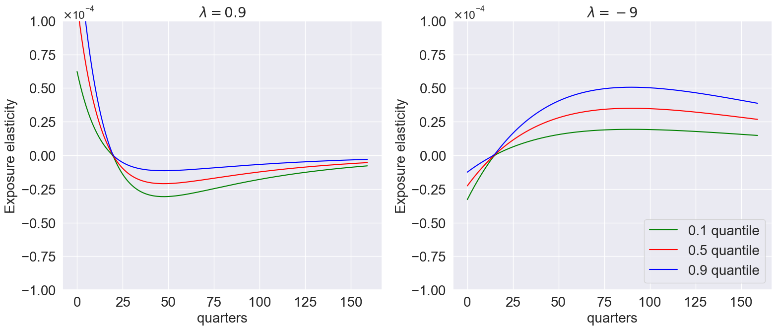
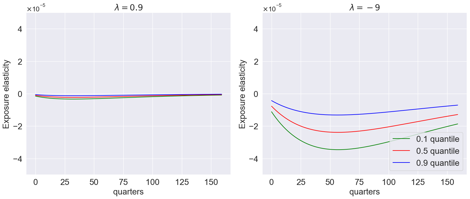
We can also illustrate exposure elasticities by varying over quantiles:

def plot_exposure_quantiles(
    model_list, 
    quantile, 
    Mtgrowth_list,
    T, 
    num_shocks, 
    time_unit='quarters', 
    ylimits=None, 
    titles=None, 
    title=None, 
    shock_names=None, 
    colors=None, 
    save_path=None
):
    """
    Plot exposure elasticity quantiles for multiple models across subplots.
    
    Parameters:
    - model_list: List of model results to plot.
    - quantile: List of quantiles to calculate.
    - T: Integer, time horizon.
    - num_shocks: Integer, number of shocks to include.
    - time_unit: String, label for x-axis time units (e.g., "quarters").
    - ylimits: List, optional y-axis limits for the subplots.
    - titles: List of titles for individual subplots.
    - title: String, optional title for the overall figure.
    - shock_names: List of strings, names for the shocks (optional, not used in this specific plot).
    - colors: List of strings, colors for the quantiles.
    - save_path: String, optional path to save the plot.
    """
    sns.set_style("darkgrid")
    num_models = len(model_list)

    # Default settings
    if titles is None:
        titles = [f'Model {i + 1}' for i in range(num_models)]
    if colors is None:
        colors = ['green', 'red', 'blue']

    # Initialize figure and axes
    fig, axes = plt.subplots(1, num_models, figsize=(8 * num_models, 7), squeeze=False)
    axes = axes.flatten()  # Flatten to ensure direct indexing works

    # Main plotting loop
    for idx, res in enumerate(model_list):
        Mtgrowth = Mtgrowth_list[idx]
        X1_tp1 = res['X1_tp1']
        X2_tp1 = res['X2_tp1']
        
        # Calculate exposure elasticity for each shock
        expo_elas_shocks = [
            [exposure_elasticity(Mtgrowth, X1_tp1, X2_tp1, T, shock=i, percentile=p) for p in quantile]
            for i in range(min(num_shocks + 1, 2))
        ]

        # Reorder shocks
        reordered_shocks = [expo_elas_shocks[1]] + [expo_elas_shocks[i] for i in range(num_shocks) if i != 1]

        # Prepare data for plotting
        index = ['T'] + [f'{q} quantile' for q in quantile]
        shock_data = [
            pd.DataFrame([np.arange(T), *[e.flatten() for e in reordered_shocks[i]]], index=index).T
            for i in range(num_shocks)
        ]

        # Plot each shock for the current model
        for i in range(num_shocks):
            for j in range(len(quantile)):
                sns.lineplot(data=shock_data[i], x='T', y=index[j + 1], ax=axes[idx], 
                             color=colors[j], label=index[j + 1])

            # Customize the subplot
            axes[idx].set_xlabel('')
            axes[idx].set_ylabel('Exposure elasticity', fontsize=20)
            axes[idx].set_title(titles[idx], fontsize=20)
            axes[idx].tick_params(axis='y', labelsize=20)
            axes[idx].tick_params(axis='x', labelsize=20)
            axes[idx].legend(fontsize=20, loc='lower right')

            # Set y-axis limits if provided
            if ylimits:
                axes[idx].set_ylim(ylimits)
            if i != 0:  # Skip the legend for the second subplot
                axes[i].legend(fontsize=15, loc='lower right')
            else:
                axes[i].legend().remove()  # Ensure no legend appears on the second plot

            # Set scientific notation for the y-axis
            axes[idx].yaxis.set_major_formatter(mticker.ScalarFormatter(useMathText=True))
            axes[idx].ticklabel_format(style='sci', axis='y', scilimits=(0, 0))


    # Set x-axis label for all subplots
    for ax in axes:
        ax.set_xlabel(f'{time_unit}', fontsize=20)

    # Set the main figure title, if provided
    if title:
        fig.suptitle(title, fontsize=24)

    plt.tight_layout()

    # Save and/or display the plot
    if save_path:
        plt.savefig(save_path, dpi=500)
    plt.show()

model_list=[
        models['gamma_1.001_lambda_0.9'],
        models['gamma_1.001_lambda_-9.0']
    ]
plot_exposure_quantiles(
    model_list,
    quantile=[0.1, 0.5, 0.9],
    Mtgrowth_list = [compute_logMtM0(model) for model in model_list],
    T=160,
    num_shocks=1,
    time_unit='quarters',
    ylimits=[-1e-4, 1e-4],
    titles=[r'$\lambda=0.9$', r'$\lambda=-9$'],
    title=None,
    # save_path='../plots/quantiles.png'      # Figure 8.7
)

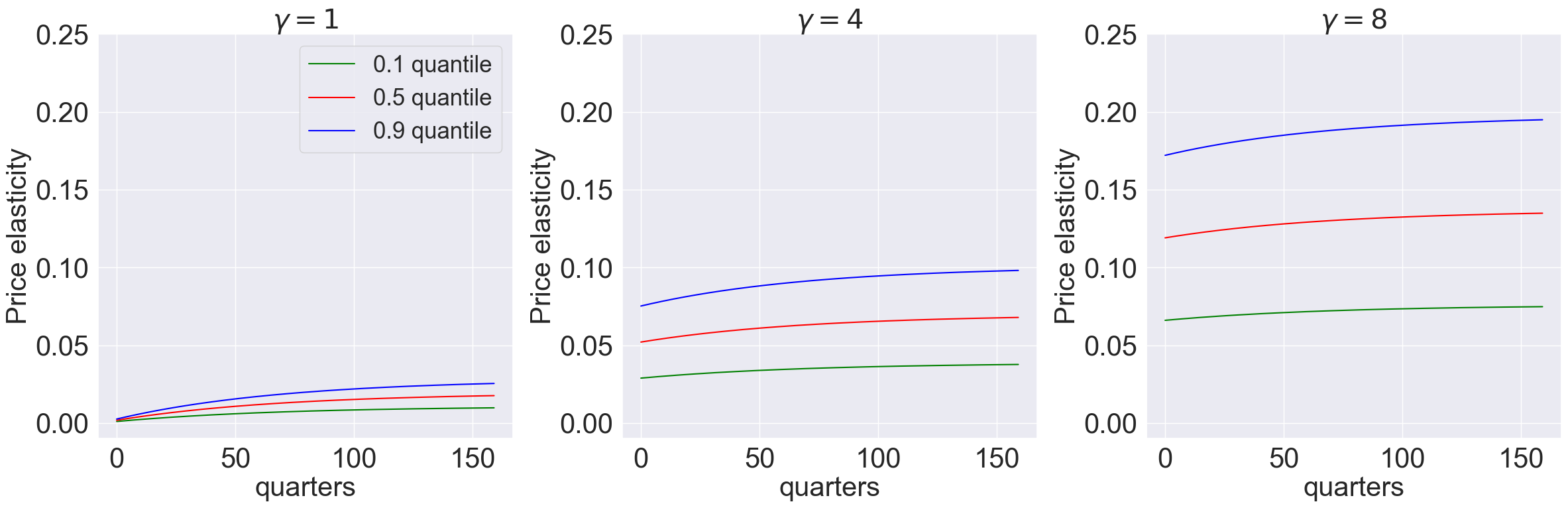
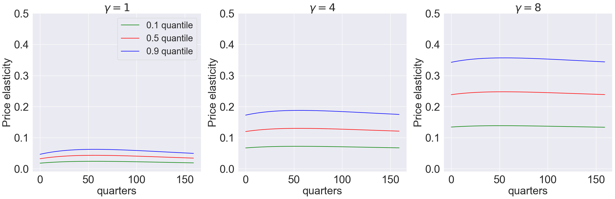
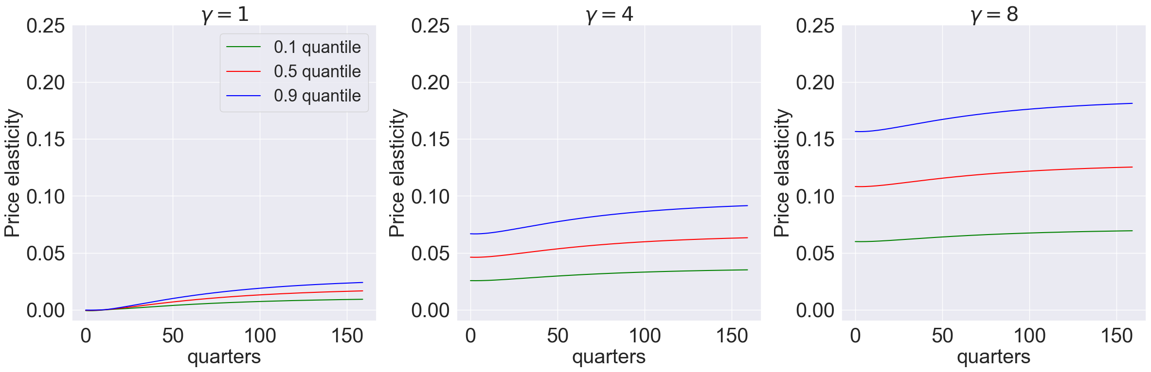
Finally we can plot price elasticities:

def plot_price_elasticity(models, T, quantile, time_unit, title=None, ylimits=None, save_path=None):
    """
    Calculate and plot price elasticity for different models across subplots.
    
    Parameters:
    - models: List of result dictionaries to plot.
    - T: Integer, time horizon.
    - quantile: List of quantiles to calculate.
    - time_unit: String, label for x-axis time units (e.g., "quarters").
    - ylimits: Optional, list of y-axis limits for each subplot.
    - save_path: Optional, path to save the figure.
    """
    sns.set_style("darkgrid")
    num_models = len(models)

    # Initialize figure and axes for subplots
    fig, axes = plt.subplots(1, num_models, figsize=(8 * num_models, 8), squeeze=False)
    axes = axes.flatten()  # Ensure axes are flattened for easy iteration
    titles = [r'$\gamma=1$',r'$\gamma=4$',r'$\gamma=8$']

    for idx, res in enumerate(models):
        # Extract data from the current model
        X1_tp1 = res['X1_tp1']
        X2_tp1 = res['X2_tp1']
        gc_tp1 = res['gc_tp1']
        vmr_tp1 = res['vmr1_tp1'] + 0.5 * res['vmr2_tp1']
        logNtilde = res['log_N_tilde']

        # Calculate log_SDF
        β = get_parameter_value('beta', res['parameter_names'], res['args'])
        ρ = get_parameter_value('rho', res['parameter_names'], res['args'])
        log_SDF = np.log(β) - ρ * gc_tp1 + (ρ - 1) * vmr_tp1 + logNtilde

        # Calculate price elasticity for each shock
        price_elas_shock = [
            price_elasticity(gc_tp1, log_SDF, X1_tp1, X2_tp1, T, shock=1, percentile=p) for p in quantile
        ]

        # Prepare data for plotting
        index = ['T'] + [f'{q} quantile' for q in quantile]
        shock_data = pd.DataFrame(
            [np.arange(T), *[e.flatten() for e in price_elas_shock]],
            index=index
        ).T

        # Plot on the respective subplot
        ax = axes[idx]
        qt = [f'{q} quantile' for q in quantile]
        colors = ['green', 'red', 'blue']

        for j in range(len(quantile)):
            sns.lineplot(data=shock_data, x='T', y=qt[j], ax=ax, color=colors[j], label=qt[j])
        
        # Customize the subplot
        ax.set_xlabel(time_unit, fontsize=30)
        ax.set_ylabel('Price elasticity', fontsize=30)
        ax.set_title(titles[idx], fontsize=30)
        ax.tick_params(axis='y', labelsize=30)
        ax.tick_params(axis='x', labelsize=30)
        if idx == 0:
            ax.legend(fontsize=25)
        else:
            ax.legend().set_visible(False)

        if ylimits:
            ax.set_ylim(ylimits)
    # plt.suptitle('$\lambda=$'+title,fontsize=35)
    plt.tight_layout()

    # Save and/or display the plot
    if save_path:
        plt.savefig(save_path, dpi=500)
    plt.show()

model_list = [models['gamma_1.001_lambda_0.0'],models['gamma_4.001_lambda_0.0'],models['gamma_8.001_lambda_0.0']]
T = 160
plot_price_elasticity(model_list,T,[0.1,0.5,0.9],'quarters','0',[-0.01,0.25]) #,r'plots/lambda0')

model_list = [models['gamma_1.001_lambda_-9.0'],models['gamma_4.001_lambda_-9.0'],models['gamma_8.001_lambda_-9.0']]
T = 160
plot_price_elasticity(model_list,T,[0.1,0.5,0.9],'quarters','-1',[-0.01,0.5]) #,r'plots/-lambda-9')

model_list = [models['gamma_1.001_lambda_0.9'],models['gamma_4.001_lambda_0.9'],models['gamma_8.001_lambda_0.9']]
T = 160
plot_price_elasticity(model_list,T,[0.1,0.5,0.9],'quarters','0.5',[-0.01,0.25]) #,r'plots/lambda09')

2.6 External Habit Model

For internal habit model, our First-order condition (FOC) is

\[ MS_t = (1 - \beta) \left(\frac {1-\lambda}{D_{1,t}} \right) + {\mathbb E} \left(N_{t+1}^* \begin{bmatrix} \frac {\beta K_t\left[1 - \exp(-\nu_h)\right]} {\exp(X_{t+1}) K_{t+1}} & 0 & 0 \end{bmatrix} MX_{t+1} \mid {\mathfrak A}_t \right) \]

For external habit, our FOC is

\[ MS_t = (1 - \beta) \left( \frac{1- \lambda}{D_{1,t}} \right) \]

In order to modify the FOC in the codes, we need to change the function compile_equations in uncertain_expansion.py. compile_equations compiles FOC and costate following

\[ \begin{align*} Q_t {\mathbb E} \left( N_{t+1} H_{t+1} \mid {\mathfrak A}_t \right) + P_t L_{t} - M_t = 0 \end{align*} \]

where

\[ \begin{align*} Q_t = & \hspace{.2cm} \beta \exp\left[(1-\rho) \left( {\widehat R}_t - {\widehat V}_t \right) \right] \cr \cr P_t = & \hspace{.2cm} (1-\beta) \exp\left[(\rho-1) \left( {\widehat V}_t - {\widehat G}_t \right) \right] \cr \cr H_{t+1} = & \hspace{.2cm} \begin{bmatrix} \psi_{d'}^x (D_t, X_t, W_{t+1})' & \psi_{d'}^g (D_t, X_t, W_{t+1}) \cr \psi_{x'}^x (D_t, X_t, W_{t+1})' & \psi_{x'}^g (D_t, X_t, W_{t+1})' \cr \psi_{g'}^x (D_t, X_t, W_{t+1})' & 1 \end{bmatrix} \begin{bmatrix} MX_{t+1} \cr MG_{t+1} \end{bmatrix} \ \cr \cr L_t = & \hspace{.2cm} \begin{bmatrix} \exp \left[ (1-\rho) \left({\widehat C}_t - {\widehat G}_t \right) \right] \begin{bmatrix} \kappa_d(D_t,X_t) \cr \kappa_x(D_t, X_t) \cr 1 \end{bmatrix} \end{bmatrix} \cr M_t = & \hspace{.2cm} \begin{bmatrix} 0 \cr MX_t \cr MG_t \end{bmatrix} + \begin{bmatrix} \phi_{d'}(D_t, X_t)' \cr \phi_{x'}(D_t,X_t)' \cr 0 \end{bmatrix} MS_t . \end{align*} \]

In our case, the \(\psi_{d'}^x (D_t, X_t, W_{t+1})\) should be \( 3 \times 2\) matrix as we have state variable \([Z_{1,t}, Z_{2,t}, X_{1,t}]\) and two controls \([\frac{I_{h,t}}{K_t}, \frac{I_{k,t}}{K_t}]\). To implement external habit model, we need the derivative of \(X_{1,t}\) process w.r.t \(\frac{I_{h,t}}{K_t}\) equal to zero.

Fortunately, we implemented this exercise and made it very easy to use for exploring the external habit model. In the equation uncertainty_expansion, when a user turns on the option ExternalHabit=True and keeps everything unchanged from the internal habit model, the code will solve the external habit model. Here is the example:

gamma_values  = [1.001, 4.001,  8.001] 
lambda_values = [-9.0,-8.0, -7.0, -6.0, -5.0, -4.0,-3.0,-2.0 ,-1.0,0.0, 0.1, 0.2, 0.3, 0.4,0.5,0.6, 0.7, 0.8, 0.9] 

initial_guess_baseline = initial_guess.copy()   # whatever you used before

preloadpath = None   # optional: external warm start (e.g. from a very easy case)

for gamma_i in gamma_values:
    # update gamma once per outer loop
    args = change_parameter_value('gamma', parameter_names, args, gamma_i)
    print(f"gamma: {gamma_i}")

    # store the last solution’s steady state for this gamma
    prev_ss = None

    for llambda_i in lambda_values:
        llambda_i = round(llambda_i, 2)
        args = change_parameter_value('llambda', parameter_names, args, llambda_i)
        print(f"lambda: {llambda_i}")

        savepath = f'output_external/res_gamma_{gamma_i}_lambda_{llambda_i}.pkl'

        # 0. If this parameter combo was already solved before, just load & move on
        if os.path.exists(savepath):
            with open(savepath, 'rb') as f:
                res = pickle.load(f)
            prev_ss = res['ss']
            print("  -> loaded existing solution from disk")
            continue

        # 1. Choose initial_guess:
        if prev_ss is not None:
            # use solution from previous λ for this γ
            initial_guess = np.concatenate([np.array([-3.40379947]), prev_ss])
        elif preloadpath is not None and os.path.exists(preloadpath):
            # optional: use some external “easy” case as a starting point
            with open(preloadpath, 'rb') as f:
                preload = pickle.load(f)
            initial_guess = np.concatenate([np.array([-3.40379947]), preload['ss']])
        else:
            # fall back to your original global guess
            initial_guess = initial_guess_baseline

        # 2. Solve at (gamma_i, llambda_i)
        res = uncertain_expansion(
            control_variables, state_variables, shock_variables,
            variables, variables_tp1,
            kappa, capital_growth, state_equations, static_constraints,
            initial_guess, parameter_names,
            args, approach='1', init_util=init_util,
            iter_tol=iter_tol, max_iter=max_iter,
            savepath=savepath,   # still writes to disk inside
            ExternalHabit=True      # <- here is the change
        )

        # 3. Store this steady state to warm-start the next λ
        prev_ss = res['ss']

        # and optionally make this the preload for future runs / sessions
        preloadpath = savepath

models = {} 
gamma_values = [1.001, 4.001,  8.001] 
lambda_values = [-9.0,   0.0,  0.9]
for gamma_i in gamma_values:
    for llambda_i in lambda_values:
        llambda_i = round(llambda_i,2)
        save_path = 'output_external/res_gamma_{}_lambda_{}.pkl'.format(gamma_i, llambda_i)
        try:
            with open(save_path, 'rb') as f:
                # models = pickle.load(save_path)
                model_key = f"gamma_{gamma_i}_lambda_{llambda_i}"
                models[model_key] = pickle.load(f)
        except FileNotFoundError:
            print(f"File not found: {save_path}")

model_list=[models['gamma_1.001_lambda_0.0'],
        models['gamma_1.001_lambda_0.9'],
        models['gamma_1.001_lambda_-9.0']]
plot_exposure_elasticity_shocks(
    model_list,
    Mtgrowth_list = [compute_logMtM0(model) for model in model_list],
    quantile=[0.5],
    T=160,
    num_shocks=2,
    time_unit='quarters',
    ylimits=[-5e-5, 5e-5],
    labels=[r'$\lambda=0$', r'$\lambda=0.9$', r'$\lambda=-9$'],
    colors=['red','green','blue'],
    title=None,
    # save_path='/plots_external/lambda_varying.png'         # Figure 10.6
)

model_list=[
        models['gamma_1.001_lambda_0.9'],
        models['gamma_1.001_lambda_-9.0']
    ]
plot_exposure_quantiles(
    model_list,
    quantile=[0.1, 0.5, 0.9],
    Mtgrowth_list = [compute_logMtM0(model) for model in model_list],
    T=160,
    num_shocks=1,
    time_unit='quarters',
    ylimits=[-5e-5, 5e-5],
    titles=[r'$\lambda=0.9$', r'$\lambda=-9$'],
    title=None,
    # save_path='/plots_external/quantiles.png'      # Figure 10.7
)

3 Outputs

3.1 List of Outputs

We now examine the contents of ModelSol, which contains the attributes listed below. Each approximation is stored in a class LinQuadVar, which contains the coefficients for \(X_{1,t}, X_{2,t}, X_{1,t}'X_{1,t}, W_{t+\epsilon}, W_{t+\epsilon}'W_{t+\epsilon}, X_{1,t}'W_{t+\epsilon}\) and the constant.

Table 3 Outputs

Input	Type	Description
JXn_t	LinQuadVar	Approximation of jump and state variables at time \(t\). Replace n with 0,1,2 to get the zeroth, first and second-order contribution. Omit n to get the full approximation. The variables are indexed in the order specified in Section 2.
Jn_t	LinQuadVar	Same as JXn_t but limited to jump variables.
Xn_tp1	LinQuadVar	Same as JXn_t but limited to state variables.
JXn_t_tilde	LinQuadVar	Same as JXn_t but using distorted measure. This variation is also available for Jn_t and Xn_tp1.
util_sol	dict	Dictionary containing solutions of the continuation values, including \(\mu^0, \Upsilon_0^2, \Upsilon_1^2,\) and \(\Upsilon_2^2\) etc.
vmrn_tp1	LinQuadVar	Approximation of continuation values \(\widehat{V}^1_{t+\epsilon}-\widehat{R}^1_t\) . Replace n with 0,1,2 to get the zeroth, first and second-order contribution. Omit n to get the full approximation.
gcn_tp1	LinQuadVar	Approximation of consumption growth \(\widehat{C}_{t+\epsilon}-\widehat{C}_t\) . Replace n with 0,1,2 to get the zeroth, first and second-order contribution. Omit n to get the full approximation.
ss	dict	Steady states for state and jump variables
log_N_tilde	LinQuadVar	Approximation for the log change of measure

For example, we can obtain the coefficients for the first-order contribution of \(\log{C_t/K_t}\) in the following way, noting that cmk_t was listed as the first jump variable when we specified the equilibrum conditions.

## Log consumption over capital approximation results, shown in the LinQuadVar coefficients form
ModelSol['JX1_t'][0].coeffs

{'x': array([[ 0.        ,  0.10420544, -0.        , -0.52822907]]),
 'c': array([[-0.0191216]])}

We can also display the full second-order approximation of \(\log{C_t/K_t}\) using the disp function, which renders a LinQuadVar object in LATEX form.

## Log consumption over capital approximation results, shown in the Latex analytical form
disp(ModelSol['JX_t'][0],'\\log\\frac{C_t}{K_t}') 

\[\begin{split}\displaystyle \log\frac{C_t}{K_t}=-3.967+\begin{bmatrix}2.53e-17&0.1082\end{bmatrix}X_t^1+\begin{bmatrix}1.242e-17&0.0521\end{bmatrix}X_t^2+X^{1T}_{t}\begin{bmatrix}6.82e-34&-1.276e-18\\1.796e-58&-5.54e-18\end{bmatrix}X^1_{t}\end{split}\]

Another example:

## Log capital growth process second order approximation results
disp(ModelSol['X2_tp1'][0],'\\log\\frac{K_{t+\epsilon}^2}{K_t^2}') 

\[\begin{split}\displaystyle \log\frac{K_{t+\epsilon}^2}{K_t^2}=-1.605e-05+\begin{bmatrix}-2.527e-21&-7.384e-06\end{bmatrix}X_t^1+\begin{bmatrix}6.824e-20&0.00987\end{bmatrix}X_t^2+X^{1T}_{t}\begin{bmatrix}-3.694e-36&6.992e-21\\-4.495e-61&3.188e-20\end{bmatrix}X^1_{t}+X^{1T}_{t}\begin{bmatrix}0&0\\0&0\end{bmatrix}W_{t+1}\end{split}\]

## Log consumption over capital approximation results, shown in the LinQuadVar coefficients form
ModelSol['JX1_t'][0].coeffs

{'x': array([[ 0.        ,  0.10420544, -0.        , -0.52822907]]),
 'c': array([[-0.0191216]])}

We can also display the full second-order approximation of \(\log{C_t/K_t}\) using the disp function, which renders a LinQuadVar object in LATEX form.

ModelSol['JX_t'][0]["x"]

array([[ 0.        ,  0.10821926, -0.0063016 , -0.52504922]])

## Log consumption over capital approximation results, shown in the Latex analytical form
disp_new(ModelSol['JX_t'][0],'\\log\\frac{C_t}{K_t}') 

\[\begin{split}\displaystyle \log\frac{C_t}{K_t}=-3.967+\begin{bmatrix}2.53e-17&0.1082&-0.006302&-0.525\end{bmatrix}X_t^1+\begin{bmatrix}1.242e-17&0.0521&5.316e-48&-0.2641\end{bmatrix}X_t^2+X^{1T}_{t}\begin{bmatrix}6.82e-34&-1.276e-18&1.79556e-58&-5.53995e-18\\-1.286e-18&-0.007021&1.11793e-55&0.0244691\\1.306e-58&-3.273e-56&-3.552e-49&-1.179e-56\\-5.633e-18&-0.05193&8.679e-58&-0.07864\end{bmatrix}X^1_{t}\end{split}\]

Another example:

## Log capital growth process second order approximation results
disp_new(ModelSol['X2_tp1'][0],'\\log\\frac{K_{t+\epsilon}^2}{K_t^2}') 

\[\begin{split}\displaystyle \log\frac{K_{t+\epsilon}^2}{K_t^2}=-1.605e-05+\begin{bmatrix}-2.527e-21&-7.384e-06&1.578e-05&4.675e-06\end{bmatrix}X_t^1+\begin{bmatrix}6.824e-20&0.00987&6.721e-62&-0.000595\end{bmatrix}X_t^2+X^{1T}_{t}\begin{bmatrix}-3.694e-36&6.992e-21&-4.49515e-61&3.18818e-20\\7.017e-21&1.032e-05&-2.79868e-58&-9.5688e-05\\-3.269e-61&8.194e-59&8.891e-52&2.953e-59\\3.212e-20&9.558e-05&-2.155e-60&5.901e-05\end{bmatrix}X^1_{t}+X^{1T}_{t}\begin{bmatrix}0&0& 0\\0&0& 0\\0.004&0.001739&0\\0&0&0\end{bmatrix}W_{t+1}\end{split}\]

3.2 Simulate Variables

Given a series of shock processes, we can simulate the path of our state and jump variables using the ModelSolution.simulate method. Here, we simulate 400 periods of i.i.d standard multivariate normal shocks.

n_J, n_X, n_W = ModelSol['var_shape']
Ws = np.random.multivariate_normal(np.zeros(n_W),np.eye(n_W),size = 400)
JX_sim = ModelSol.simulate(Ws)

4 Using LinQuadVar in Computation

In the previous section, we saw how to use uncertain_expansion to approximate variables and store their coefficients as LinQuadVar objects. In this section, we explore how to manipulate LinQuadVar objects for different uses.

To aid our examples, we first extract the steady states for the state evolution processes from the previous model solution:

See src/lin_quad.py for source code of LinQuadVar definition.

ModelSol['ss'][[0,1,2]]

array([-4.33215389,  0.0259344 ,  0.02039568])

n_J, n_X, n_W = ModelSol['var_shape']
print(n_J, n_X, n_W)
X0_tp1 = LinQuadVar({'c':np.array([[ModelSol['ss'][0]],[ModelSol['ss'][1]],[ModelSol['ss'][2]], [ModelSol["ss"][3]]])}, shape = (n_X, n_X, n_W))

6 4 3

4.1 LinQuadVar Operations

We can sum multiple LinQuads together in two different ways. Here we demonstrate this with an example by summing the zeroth, first and second order contributions of our approximation for capital growth.

gk_tp1 = X0_tp1[0] + ModelSol['X1_tp1'][0]  + 0.5 * ModelSol['X2_tp1'][0] 
disp(gk_tp1,'\\log\\frac{K_{t+\epsilon}}{K_t}') 

\[\begin{split}\displaystyle \log\frac{K_{t+\epsilon}}{K_t}=-4.331+\begin{bmatrix}-1.258e-18&0.03725\end{bmatrix}X_t^1+\begin{bmatrix}0.007999&0.003478\end{bmatrix}W_{t+1}+\begin{bmatrix}-6.64e-19&0.01855\end{bmatrix}X_t^2+X^{1T}_{t}\begin{bmatrix}-3.805e-34&-4.484e-19\\2.307e-60&4.654e-21\end{bmatrix}X^1_{t}+X^{1T}_{t}\begin{bmatrix}0&0\\0&0\end{bmatrix}W_{t+1}\end{split}\]

In the next example, we sum together the contributions for both capital growth and technology:

lq_sum([X0_tp1, ModelSol['X1_tp1'], 0.5 * ModelSol['X2_tp1']]).coeffs

{'xx': array([[-0.        , -0.        ,  0.        ,  0.        ,  0.        , -0.00022514,  0.        ,  0.00001292,  0.        ,  0.        , -0.        ,  0.        ,  0.        ,  0.00001093,
          0.        , -0.00003523],
        [ 0.        ,  0.        ,  0.        ,  0.        ,  0.        ,  0.        ,  0.        ,  0.        ,  0.        ,  0.        ,  0.        ,  0.        ,  0.        ,  0.        ,
          0.        ,  0.        ],
        [ 0.        ,  0.        ,  0.        ,  0.        ,  0.        ,  0.        ,  0.        ,  0.        ,  0.        ,  0.        ,  0.097     ,  0.        ,  0.        ,  0.        ,
          0.        ,  0.        ],
        [ 0.        ,  0.        , -0.        ,  0.        , -0.        ,  0.00025426, -0.        ,  0.00000844, -0.        , -0.        ,  0.        , -0.        ,  0.        ,  0.00001072,
         -0.        ,  0.00005381]]),
 'c': array([[-4.33102269],
        [ 0.0259344 ],
        [-0.07112813],
        [-0.00131024]]),
 'w': array([[ 0.00799924,  0.00347793,  0.        ],
        [ 0.        ,  0.04956051,  0.        ],
        [ 0.        ,  0.        ,  0.42784065],
        [-0.00799924, -0.00347793,  0.        ]]),
 'x': array([[-0.        ,  0.03724612,  0.00008824,  0.00005908],
        [ 0.        ,  0.944     ,  0.        ,  0.        ],
        [ 0.        ,  0.        ,  0.806     ,  0.        ],
        [ 0.        , -0.03682226, -0.00010169, -0.10517424]]),
 'xw': array([[ 0.        ,  0.        ,  0.        ,  0.        ,  0.        ,  0.        ,  0.00399962,  0.00173897,  0.        ,  0.        ,  0.        ,  0.        ],
        [ 0.        ,  0.        ,  0.        ,  0.        ,  0.        ,  0.        ,  0.        ,  0.02478025,  0.        ,  0.        ,  0.        ,  0.        ],
        [ 0.        ,  0.        ,  0.        ,  0.        ,  0.        ,  0.        ,  0.        ,  0.        , -0.21392032,  0.        ,  0.        ,  0.        ],
        [ 0.        ,  0.        ,  0.        ,  0.        ,  0.        ,  0.        , -0.00399962, -0.00173897,  0.        ,  0.        ,  0.        ,  0.        ]]),
 'x2': array([[-0.        ,  0.01855206, -0.        ,  0.00003412],
        [ 0.        ,  0.472     ,  0.        ,  0.        ],
        [ 0.        ,  0.        ,  0.403     ,  0.        ],
        [ 0.        , -0.0183313 ,  0.        , -0.05258344]])}

4.2 LinQuadVar Split and Concat

split breaks multiple dimensional LinQuad into one-dimensional LinQuads, while concat does the inverse.

gk_tp1, Z_tp1, Y_tp1, X_tp1 = ModelSol['X1_tp1'].split()
concat([gk_tp1, Z_tp1, Y_tp1])

<lin_quad.LinQuadVar at 0x25f969bd8b0>

4.3 Evaluate a LinQuadVar

We can evaluate a LinQuad at specific state \((X_{t},W_{t+\epsilon})\) in time. As an example, we evaluate all 5 variables under steady state with a multivariate random normal shock.

x1 = np.zeros([n_X ,1])
x2 = np.zeros([n_X ,1])
x3 = np.zeros([n_X, 1])
w = np.random.multivariate_normal(np.zeros(n_W),np.eye(n_W),size = 1).T
ModelSol['JX_tp1'](*(x1,x2,w))

array([[ -4.40157174],
       [  0.02420615],
       [  0.02040907],
       [ -0.0002646 ],
       [ -0.00021192],
       [  0.99999632],
       [  0.02218119],
       [  0.01258757],
       [-12.16998153],
       [ -0.01876417]])

4.4 Next period expression for LinQuadVar

ModelSol allows us to express a jump variable \(J_t\) as a function of \(t\) state and shock variables. Suppose we would like to compute its next period expression \(J_{t+\epsilon}\) with shocks. The function next_period expresses \(J_{t+\epsilon}\) in terms of \(t\) state variables and \(t+\epsilon\) shock variables. For example, we can express the \(t+\epsilon\) expression for the first-order contribution to consumption over capital as:

ModelSol["X1_tp1"].coeffs

{'x': array([[-0.        ,  0.03710412, -0.        ,  0.00006824],
        [-0.        ,  0.944     , -0.        , -0.        ],
        [-0.        , -0.        ,  0.806     , -0.        ],
        [ 0.        , -0.0366626 ,  0.        , -0.10516689]]),
 'w': array([[ 0.00799924,  0.00347793, -0.        ],
        [-0.        ,  0.04956051, -0.        ],
        [-0.        , -0.        ,  0.42784065],
        [-0.00799924, -0.00347793, -0.        ]]),
 'c': array([[ 0.00111162],
        [ 0.        ],
        [ 0.        ],
        [-0.0012811 ]])}

cmk1_tp1 = next_period(ModelSol['J1_t'][0], ModelSol['X1_tp1'])
disp(cmk1_tp1, '\\log\\frac{C_{t+\epsilon}^1}{K_{t+\epsilon}^1}') 

\[\displaystyle \log\frac{C_{t+\epsilon}^1}{K_{t+\epsilon}^1}=-0.06643+\begin{bmatrix}-2.655e-20&0.1641\end{bmatrix}X_t^1+\begin{bmatrix}0.0001387&0.00864\end{bmatrix}W_{t+1}\]

cmk2_tp1 = next_period(ModelSol['J2_t'][0], ModelSol['X1_tp1'], ModelSol['X2_tp1'])
disp(cmk2_tp1, '\\log\\frac{C_{t+\epsilon}^2}{K_{t+\epsilon}^2}') 

\[\begin{split}\displaystyle \log\frac{C_{t+\epsilon}^2}{K_{t+\epsilon}^2}=-0.01178+\begin{bmatrix}6.104e-21&0.007963\end{bmatrix}X_t^1+\begin{bmatrix}-1.769e-05&0.0004143\end{bmatrix}W_{t+1}+\begin{bmatrix}-2.655e-20&0.1641\end{bmatrix}X_t^2+X^{1T}_{t}\begin{bmatrix}-1.513e-35&-2.292e-20\\9.225e-62&-3.041e-21\end{bmatrix}X^1_{t}+X^{1T}_{t}\begin{bmatrix}-4.345e-22&-6.35e-22\\2.099e-76&5.481e-05\end{bmatrix}W_{t+1}+W_{t+1}^{T}\begin{bmatrix}1.135e-06&1.612e-06\\-9.439e-61&1.706e-06\end{bmatrix}W_{t+1}\end{split}\]

4.6 Compute the Expectation of time \(t+\epsilon\) LinQuadVar

Suppose the distribution of shocks has a constant mean and variance (not state dependent). Then, we can use the E function to compute the expectation of a time \(t+\epsilon\) LinQuadVar as follows:

E_w = ModelSol['util_sol']['μ_0']
cov_w = np.eye(n_W)
E_ww = cal_E_ww(E_w, cov_w)
E_cmk2_tp1 = E(cmk2_tp1, E_w, E_ww)
disp(E_cmk2_tp1, '\mathbb{E}[\\log\\frac{C_{t+\epsilon}^2}{K_{t+\epsilon}^2}|\mathfrak{F_t}]')

\[\begin{split}\displaystyle \mathbb{E}[\log\frac{C_{t+\epsilon}^2}{K_{t+\epsilon}^2}|\mathfrak{F_t}]=-0.01189+\begin{bmatrix}6.265e-21&0.008079\end{bmatrix}X_t^1+\begin{bmatrix}-2.655e-20&0.1641\end{bmatrix}X_t^2+X^{1T}_{t}\begin{bmatrix}-1.513e-35&-2.292e-20\\9.225e-62&-3.041e-21\end{bmatrix}X^1_{t}\end{split}\]

Suppose the distribution of shock has a state-dependent mean and variance (implied by \(\tilde{N}_{t+\epsilon}\) shown in the notes), we can use E_N_tp1 and N_tilde_measure to compute the expectation of time \(t+\epsilon\) LinQuadVar.

N_cm = N_tilde_measure(ModelSol['util_sol']['log_N_tilde'],(1,n_X,n_W))
E_cmk2_tp1_tilde = E_N_tp1(cmk2_tp1, N_cm)
disp(E_cmk2_tp1_tilde, '\mathbb{\\tilde{E}}[\\log\\frac{C_{t+\epsilon}^2}{K_{t+\epsilon}^2}|\mathfrak{F_t}]')

\[\begin{split}\displaystyle \mathbb{\tilde{E}}[\log\frac{C_{t+\epsilon}^2}{K_{t+\epsilon}^2}|\mathfrak{F_t}]=-0.01211+\begin{bmatrix}6.267e-21&0.008083\end{bmatrix}X_t^1+\begin{bmatrix}-2.655e-20&0.1641\end{bmatrix}X_t^2+X^{1T}_{t}\begin{bmatrix}-1.513e-35&-2.292e-20\\4.009e-25&-3.041e-21\end{bmatrix}X^1_{t}\end{split}\]