Notebook: Expansion Suite

Notebook: Expansion Suite #

We previously covered the small-noise expansion method and the recursive utility framework. This section covers the usage of Expansion Suite, an open source Python toolbox which uses these methods to solve discrete nonlinear DSGE models.

This notebook provides both written explanations and accompanying code. The simplest way to run the code is to open the Google Colab link at the top of this page. Otherwise, the reader can copy the code snippets onto their local machine.

Consider the framework previously introduced:

\[\begin{split} \begin{align} \mathbb{E}[{N_{t+1}^*Q_{t+1}^* \psi_1(X_t, J_t, X_{t+1}, J_{t+1})}|{\mathfrak{A}_t}] - \psi_2(X_t, J_t) &= 0 \tag{1}\\ \phi\left(X_t, X_{t+1}, J_t, {\sf q}W_{t+1}, {\sf q} \right) &= 0 \tag{2} \end{align} \end{split}\]

The Expansion Suite uses the function uncertain_expansion to approximate a solution to the above system locally. It takes the following inputs:

Input	Type	Description
`eq`	callable	Function which takes state and jump variables and outputs error of equilibrium conditions, i.e. RHS of equation (1)
`ss`	callable	Function which takes model parameters and outputs steady-state values of state and jump variables
`var_shape`	tuple of int	Triple of integers \((n_J,n_X,n_W)\) where \(n_J\) is the number of jump variables, \(n_X\) is the number of state variables, and \(n_W\) is the number of shocks.
`args`	tuple of float or ndarray	Array of preference and model parameters
`gc`	callable	Function which takes in variables and outputs log-growth of consumption
`args`	tuple of float/ndarray	Preference and model parameters
`gc`	callable	Function which takes in variables and outputs log-growth of consumption
`approach`	string	If equal to ‘1’, then solve the model using approach 1 (default, see Appendix C); If equal to ‘2’, then use approach 2 (see Appendix D). The function raises an exception if other values are provided
`init_util`	dict, or None	Dictionary for initialization of the expansion coefficients \(\mu^0, \Upsilon_0^2, \Upsilon_1^2,\) and \(\Upsilon_2^2\). The keys are: `mu_0`, `Upsilon_0`, `Upsilon_1`, `Upsilon_2`. If None, zero matrices are used
`iter_tol`	float	Iteration stops when the maximum absolute difference between the approximated variables in the current and previous iteration is below `iter_tol`
`max_iter`	int	Maximum number of iterations

The output is of class ModelSolution, which stores the coefficients for the linear-quadratic approximation for the jump and state variables; continuation values; consumption growth; and log change of measure, as well as the steady-state values of each variables.

We will now walk through the computation using a simple example.

1 AK Model with Recursive Utility #

1.1 Model Setup #

Consider the following recursive utility maximization problem with AK technology:

\[ \max_{C_t, I_t} V_t = \left[ (1 - \beta) \left(C_t\right)^{1-\rho} + \beta \left( R_t \right)^{1-\rho} \right]^{\frac 1 {1-\rho}}\tag{3} \]

such that

\[ C_t + I_t = \alpha K_t \]

\[ \log K_{t+1} - \log K_t = \frac 1 \psi \log \left[ 1 + \psi \frac {I_t}{K_t} \right] + \beta_k Z_t - \eta_k + \sigma_k W_{t+1} \]

\[ Z_{t+1} = \exp( - \beta_z) Z_t + \sigma_z W_{t+1} \]

where \(\psi\) is adjustment cost parameter which determines the efficiency of converting investment to capital, and \(\eta_k\) is depreciation. \(Z_t\) governs the (scalar) conditional mean of (stochastic) technology growth while \(\sigma_k\) governs the stochastic volatility of technology growth. \(W_{t+1}\) is a two-dimensional Wiener process which provides the exogenous shocks to this model.

For the purposes of computation, we divide the first two equations by \(K_t\).

1.2 First-Order Conditions #

Let \({\widehat G}_t = {\widehat K}_t,\) \(X_t = Z_t,\) and \(D_t = \frac {I_t }{K_t}.\) We can rewrite the previous equations as:

\[ {\widehat C}_t = \log \left( \alpha - D_t \right) + {\widehat G}_t \]

\[ {\widehat G}_{t + 1} - {\widehat G}_t = \frac 1 \psi \log \left[ 1 + \psi D_t \right] + \beta_k X_t - \eta_k + \sigma_k W_{t+1} \]

Apply the general form of FOC and costate equations and notice in this special case \(\psi^x_d = 0\), we have

The FOC is

\[ \mathbb{E} \left[N^*_{t + 1}Q^*_{t + 1} \beta \left(\frac{C_{t + 1}}{G_{t + 1}}\right)^{-\rho} \left(\frac{G_{t + 1}}{G_{t}}\right)^{1-\rho} \left(\frac{C_{t}}{G_{t}}\right)^{\rho} \frac{1}{1 + \psi D_t} \widetilde{MG}_{t+1} \right] - 1 = 0 \]

The law of motion of costate \(\widetilde{MG}\) is

\[ \mathbb{E} \left[N^*_{t + 1}Q^*_{t + 1} \beta \left(\frac{C_{t + 1}}{G_{t + 1}}\right)^{-\rho} \left(\frac{G_{t + 1}}{G_{t}}\right)^{1-\rho} \left(\frac{C_{t}}{G_{t}}\right)^{\rho} \widetilde{MG}_{t+1} \right ] - \widetilde{MG}_t + \frac{C_t}{G_t} = 0 \]

Finally, we can express our system of equations as

\[\begin{split} \psi_1 = \begin{bmatrix} 0\\ \beta \left(\frac{C_{t + 1}}{G_{t + 1}}\right)^{-\rho} \left(\frac{G_{t + 1}}{G_{t}}\right)^{1-\rho} \left(\frac{C_{t}}{G_{t}}\right)^{\rho} \frac{1}{1 + \psi D_t} \widetilde{MG}_{t+1} \\ \beta \left(\frac{C_{t + 1}}{G_{t + 1}}\right)^{-\rho} \left(\frac{G_{t + 1}}{G_{t}}\right)^{1-\rho} \left(\frac{C_{t}}{G_{t}}\right)^{\rho} \widetilde{MG}_{t+1} \end{bmatrix} \end{split}\]

\[\begin{split} \psi_2 = \begin{bmatrix} \frac{C_t}{G_t} + D_t - {\mathbf a}\\ 1\\ \widetilde{MG}_t - \frac{C_t}{G_t} \end{bmatrix} \end{split}\]

\[\begin{split}\phi=\begin{bmatrix} &\frac{G_{t+1}} {G_t} - \left( 1 + \psi D_t \right)^{\frac{1}{\psi}} + exp( \beta_k Z_t - \eta_k + \sigma_k W_{t+1} ) \\ &Z_{t+1} - \exp( - \beta_z) Z_t - \sigma_z W_{t+1} \end{bmatrix}\end{split}\]

The model has thre e jump variables (In the expansion suite, \(J_t\) is used to represent the array of jump variables):

\(\log C_t - \log G_t\) : Log consumption over capital
\(\log D_t\) : Log investment over capital
\(\log MG_t\) : Log co-state variable

and two state variables (In the expansion suite, \(X_t\) is used to represent state variables):

\(\log G_{t} - \log G_{t-1}\) : Log capital growth process
\(Z_{t}\) : Exogenous technology

2 Inputs #

2.1 Libraries #

Begin by installing the following libraries and downloading RiskUncertaintyValue, which contains the functions required to solve the model:

import os
import sys
workdir = os.getcwd()
!git clone https://github.com/lphansen/RiskUncertaintyValue 
workdir = os.getcwd() + '/RiskUncertaintyValue'             
sys.path.insert(0, workdir+'/src')                        
import numpy as np
import autograd.numpy as anp
from scipy import optimize
np.set_printoptions(suppress=True)
np.set_printoptions(linewidth=200)
from IPython.display import display, HTML
from BY_example_sol import disp
display(HTML("<style>.container { width:97% !important; }</style>"))
import warnings
warnings.filterwarnings("ignore")

from lin_quad import LinQuadVar
from lin_quad_util import E, concat, next_period, cal_E_ww, lq_sum, N_tilde_measure, E_N_tp1
from uncertain_expansion import uncertain_expansion
np.set_printoptions(suppress=True)

fatal: destination path 'RiskUncertaintyValue' already exists and is not an empty directory.

2.2 Equilibrium Condition Function #

The first input for uncertain_expansion requires us to define the equilibrium conditions for the model. Therefore we define a function eq which takes in a list of jump and state variables as inputs, and outputs the equilibrium equations in the form of equations 1 and 2. The inputs required:

Variable	Type	Description	Corresponds to
`Var_t`	array-like	Vector of jump and state variables in the current period	\((J_t, X_t)\)
`Var_tp1`	array-like	Vector of jump and state variables in the next period	\((J_{t+1}, X_{t+1})\)
`W_tp1`	array-like	Vector of shock variables in the next period	\((W_{t+1})\)
`q`	float	Perturbation parameter	\(q\)
`mode`	string	By default, this function returns the LHS of equation (1) and (2). Set mode to ‘psi1’, ‘psi2’, or ‘phi’ to return the corresponding function in the equilibrium conditions
`args`	tuple of float/ndarray	Preference and model parameters

While writing out eq, ensure that:

The first components of Var_t and Var_tp1 are fixed as q_t or q_tp1.
State variables follow jump variables.
The number of jump variables (except q_t and q_tp1) equals the number of forward-looking equilibrium conditions.
The number of state variables equals to the number of state evolution equations.
All values are expressed as type float. Otherwise, this may cause type errors.

Note that the log change of measure is skipped in the specification of equilibrium conditions.

Notice that the first 3 parameters and \(q\) in variables should be defined and called in the given order.

For the example model, we write:

2.3 Steady State Function #

This function takes model parameters as input and outputs the steady states for each variable following the variable order specified in Var_t and Var_tp1. To find the steady state, we remove the time subscripts from each variable and solve the system of equations.

Note that the first entry of the output array will always be 0, since the steady state of q_t is 0.

2.4 Specifying Number of Variables #

We need to specify the number of jump variables, state and shock variables as an array (n_J, n_X, n_W).

2.5 Model Parameters #

Next, we need to specify all the model parameters using a Python tuple.

The first three parameters should be γ, β, ρ, respectively. The package is designed for recursive utlity.
Please use 1.00001 for γ and ρ as approximation for 1.0.
We suggest not using matrix when specifying the equilibrium conditions and parameters.

2.6 Log Consumption Growth #

Finally, we need to specify how to compute the log-growth of consumption \(\log{C_{t+1}/C_t}\) using the defined variables Var_t and Var_tp1 in the equilibrium conditions.

In this example, we simply use the decomposition:

\[ \log{C_{t+1}/C_t} = \log{C_{t+1}/K_{t+1}} + \log{K_{t+1}/K_t} - \log{C_t/K_t} \]

The reason to specify log consumtion growth is that we need to approximate recursive utility as described in the notes section 3.2.2 and section 3.2.3
In habit formation models, \(C_t\) is replaced with \(U_t\), in which case we would specify the log growth process for \(U_t\) correspondingly.

2.7 Computing ModelSol #

Now we are able to use steps 2.1 to 2.5 as inputs to the uncertain_expansion function. The solution is stored in a class named ModelSolution(Please refer to uncertainexpansion.ipynb for details.) under the Linear Quadratic Framework.

See src/uncertain_expansion.py for the source code of the expansion suite.

3 Outputs #

3.1 List of Outputs #

We now examine the contents of ModelSol, which contains the attributes listed below. Each approximation is stored in a class LinQuadVar, which contains the coefficients for \(X_{1,t}, X_{2,t}, X_{1,t}'X_{1,t}, W_{t+1}, W_{t+1}'W_{t+1}, X_{1,t}'W_{t+1}\) and the constant.

Input	Type	Description
`JXn_t`	LinQuadVar	Approximation of jump and state variables at time \(t\). Replace `n` with `0,1,2` to get the zeroth, first and second-order contribution. Omit `n` to get the full approximation. The variables are indexed in the order specified in Section 2.
`Jn_t`	LinQuadVar	Same as `JXn_t` but limited to jump variables.
`Xn_tp1`	LinQuadVar	Same as `JXn_t` but limited to state variables.
`JXn_t_tilde`	LinQuadVar	Same as `JXn_t` but using distorted measure. This variation is also available for `Jn_t` and `Xn_tp1`.
`util_sol`	dict	Dictionary containing solutions of the continuation values, including \(\mu^0, \Upsilon_0^2, \Upsilon_1^2,\) and \(\Upsilon_2^2\) etc.
`vmrn_tp1`	LinQuadVar	Approximation of continuation values \(\widehat{V}^1_{t+1}-\widehat{R}^1_t\) . Replace `n` with `0,1,2` to get the zeroth, first and second-order contribution. Omit `n` to get the full approximation.
`gcn_tp1`	LinQuadVar	Approximation of consumption growth \(\widehat{C}_{t+1}-\widehat{C}_t\) . Replace `n` with `0,1,2` to get the zeroth, first and second-order contribution. Omit `n` to get the full approximation.
`ss`	dict	Steady states for state and jump variables
`log_N_tilde`	LinQuadVar	Approximation for the log change of measure

For example, we can obtain the coefficients for the first-order contribution of \(\log{C_t/K_t}\) in the following way, noting that cmk_t was listed as the first jump variable when we specified the equilibrum conditions.

## Log consumption over capital approximation results, shown in the LinQuadVar coefficients form
ModelSol['JX1_t'][0].coeffs

{'c': array([[-0.02117949]]), 'x': array([[ 0.04344641, -0.        ]])}

We can also display the full second-order approximation of \(\log{C_t/K_t}\) using the disp function, which renders a LinQuadVar object in LATEX form.

## Log consumption over capital approximation results, shown in the Latex analytical form
disp(ModelSol['JX_t'][0],'\\log\\frac{C_t}{K_t}') 

\[\begin{split}\displaystyle \log\frac{C_t}{K_t}=-3.683+\begin{bmatrix}0.04379&-1.599e-18\end{bmatrix}X_t^1+\begin{bmatrix}0.02172&-7.979e-19\end{bmatrix}X_t^2+X^{1T}_{t}\begin{bmatrix}-0.0002216&6.006e-20\\-5.324e-20&-2.217e-36\end{bmatrix}X^1_{t}\end{split}\]

Another example:

## Log capital growth process second order approximation results
disp(ModelSol['X2_tp1'][0],'\\log\\frac{K_{t+1}^2}{K_t^2}') 

\[\displaystyle \log\frac{K_{t+1}^2}{K_t^2}=\begin{bmatrix}0.9455&-0\end{bmatrix}X_t^2\]

3.3 Simulate Variables #

Given a series of shock processes, we can simulate the path of our state and jump variables using the ModelSolution.simulate method. Here, we simulate 400 periods of i.i.d standard multivariate normal shocks.

Ws = np.random.multivariate_normal(np.zeros(n_W),np.eye(n_W),size = 400)
JX_sim = ModelSol.simulate(Ws)

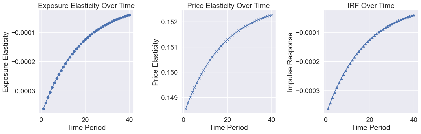
3.4 Shock Elasticities and IRF #

ModelSolution contains a method elasticities used to compute the shock elasticities of jump and state variables. We do this by defining a log_SDF_ex function, which expresses the log stochastic discount factor exclusive of the change of measure \({N}^*_{t+1}\) and variable \(Q_{t+1}^*\). Shock elasticities are great tools for nonlinear impulsive response analyses, and in linear models, the shock elasticities correspond to the traditional impulse response function (IRF).

ModelSolution also has a method IRF to compute the traditional IRF of all jump and state variables. Below we calculate the IRF of all variables with respect to the first shock for 400 periods.

The figure plots elasticities and IRF of investment rate with regard to shock 1.

4 Using `LinQuadVar` in Computation #

In the previous section, we saw how to use uncertain_expansion to approximate variables and store their coefficients as LinQuadVar objects. In this section, we explore how to manipulate LinQuadVar objects for different uses.

To aid our examples, we first extract the steady states for the state evolution processes from the previous model solution:

See src/lin_quad.py for source code of LinQuadVar definition.

n_J, n_X, n_W = ModelSol['var_shape']
X0_tp1 = LinQuadVar({'c':np.array([[ModelSol['ss'][1]],[ModelSol['ss'][2]]])}, shape = (2, n_X, n_W))
X0_tp1.coeffs

{'c': array([[-2.71057934],
        [ 1.5576879 ]])}

4.1 `LinQuadVar` Operations #

We can sum multiple LinQuads together in two different ways. Here we demonstrate this with an example by summing the zeroth, first and second order contributions of our approximation for capital growth.

gk_tp1 = X0_tp1[0] + ModelSol['X1_tp1'][0]  + 0.5 * ModelSol['X2_tp1'][0] 
disp(gk_tp1,'\\log\\frac{K_{t+1}}{K_t}') 

\[\displaystyle \log\frac{K_{t+1}}{K_t}=-2.711+\begin{bmatrix}0.9455&0\end{bmatrix}X_t^1+\begin{bmatrix}0.022&0.05\end{bmatrix}W_{t+1}+\begin{bmatrix}0.4728&0\end{bmatrix}X_t^2\]

In the next example, we sum together the contributions for both capital growth and technology:

lq_sum([X0_tp1, ModelSol['X1_tp1'], 0.5 * ModelSol['X2_tp1']]).coeffs

{'c': array([[-2.71057934],
        [ 1.55804585]]),
 'x': array([[0.94553914, 0.        ],
        [0.00928281, 0.        ]]),
 'w': array([[0.022  , 0.05   ],
        [0.00954, 0.     ]]),
 'x2': array([[0.47276957, 0.        ],
        [0.00463556, 0.        ]]),
 'xx': array([[ 0.        ,  0.        ,  0.        ,  0.        ],
        [-0.00001424, -0.        ,  0.        ,  0.        ]])}

4.2 `LinQuadVar` Split and Concat #

split breaks multiple dimensional LinQuad into one-dimensional LinQuads, while concat does the inverse.

gk_tp1, Z_tp1 = ModelSol['X1_tp1'].split()
concat([gk_tp1, Z_tp1])

<lin_quad.LinQuadVar at 0x7fd482a310d0>

4.3 Evaluate a `LinQuadVar` #

We can evaluate a LinQuad at specific state \((X_{t},W_{t+1})\) in time. As an example, we evaluate all 5 variables under steady state with a multivariate random normal shock.

x1 = np.zeros([n_X ,1])
x2 = np.zeros([n_X ,1])
w = np.random.multivariate_normal(np.zeros(n_W),np.eye(n_W),size = 1).T
ModelSol['JX_tp1'](*(x1,x2,w))

array([[-3.68477708],
       [-2.70160922],
       [ 1.56188201],
       [-0.04541874],
       [ 0.03643626]])

4.4 Next period expression for `LinQuadVar` #

ModelSol allows us to express a jump variable \(J_t\) as a function of \(t\) state and shock variables. Suppose we would like to compute its next period expression \(J_{t+1}\) with shocks. The function next_period expresses \(J_{t+1}\) in terms of \(t\) state variables and \(t+1\) shock variables. For example, we can express the \(t+1\) expression for the first-order contribution to consumption over capital as:

cmk1_tp1 = next_period(ModelSol['J1_t'][0], ModelSol['X1_tp1'])
disp(cmk1_tp1, '\\log\\frac{C_{t+1}^1}{K_{t+1}^1}') 

\[\displaystyle \log\frac{C_{t+1}^1}{K_{t+1}^1}=-0.02118+\begin{bmatrix}0.04108&-4.272e-38\end{bmatrix}X_t^1+\begin{bmatrix}0.0009558&0.002172\end{bmatrix}W_{t+1}\]

cmk2_tp1 = next_period(ModelSol['J2_t'][0], ModelSol['X1_tp1'], ModelSol['X2_tp1'])
disp(cmk2_tp1, '\\log\\frac{C_{t+1}^2}{K_{t+1}^2}') 

\[\begin{split}\displaystyle \log\frac{C_{t+1}^2}{K_{t+1}^2}=-0.0008222+\begin{bmatrix}0.0006544&1.696e-39\end{bmatrix}X_t^1+\begin{bmatrix}1.523e-05&3.46e-05\end{bmatrix}W_{t+1}+\begin{bmatrix}0.04108&-4.272e-38\end{bmatrix}X_t^2+X^{1T}_{t}\begin{bmatrix}-0.0003962&4.152e-39\\-7.651e-39&-4.137e-56\end{bmatrix}X^1_{t}+X^{1T}_{t}\begin{bmatrix}-1.844e-05&-4.191e-05\\8.042e-42&1.828e-41\end{bmatrix}W_{t+1}+W_{t+1}^{T}\begin{bmatrix}-2.145e-07&-4.875e-07\\-4.875e-07&-1.108e-06\end{bmatrix}W_{t+1}\end{split}\]

4.6 Compute the Expectation of time \(t+1\) `LinQuadVar` #

Suppose the distribution of shocks has a constant mean and variance (not state dependent). Then, we can use the E function to compute the expectation of a time \(t+1\) LinQuadVar as follows:

E_w = ModelSol['util_sol']['μ_0']
cov_w = np.eye(n_W)
E_ww = cal_E_ww(E_w, cov_w)
E_cmk2_tp1 = E(cmk2_tp1, E_w, E_ww)
disp(E_cmk2_tp1, '\mathbb{E}[\\log\\frac{C_{t+1}^2}{K_{t+1}^2}|\mathfrak{F_t}]')

\[\begin{split}\displaystyle \mathbb{E}[\log\frac{C_{t+1}^2}{K_{t+1}^2}|\mathfrak{F_t}]=-0.0008284+\begin{bmatrix}0.0006602&1.694e-39\end{bmatrix}X_t^1+\begin{bmatrix}0.04108&-4.272e-38\end{bmatrix}X_t^2+X^{1T}_{t}\begin{bmatrix}-0.0003962&4.152e-39\\-7.651e-39&-4.137e-56\end{bmatrix}X^1_{t}\end{split}\]

Suppose the distribution of shock has a state-dependent mean and variance (implied by \(\tilde{N}_{t+1}\) shown in the notes), we can use E_N_tp1 and N_tilde_measure to compute the expectation of time \(t+1\) LinQuadVar.

N_cm = N_tilde_measure(ModelSol['util_sol']['log_N_tilde'],(1,n_X,n_W))
E_cmk2_tp1_tilde = E_N_tp1(cmk2_tp1, N_cm)
disp(E_cmk2_tp1_tilde, '\mathbb{\\tilde{E}}[\\log\\frac{C_{t+1}^2}{K_{t+1}^2}|\mathfrak{F_t}]')

\[\begin{split}\displaystyle \mathbb{\tilde{E}}[\log\frac{C_{t+1}^2}{K_{t+1}^2}|\mathfrak{F_t}]=-0.0008284+\begin{bmatrix}0.0006602&1.694e-39\end{bmatrix}X_t^1+\begin{bmatrix}0.04108&-4.272e-38\end{bmatrix}X_t^2+X^{1T}_{t}\begin{bmatrix}-0.0003963&4.152e-39\\-7.651e-39&-4.137e-56\end{bmatrix}X^1_{t}\end{split}\]

Notebook: Expansion Suite

Contents

Notebook: Expansion Suite#

1 AK Model with Recursive Utility#