1. Stochastic Processes and Laws of Large Numbers

1.1. Introduction

A probabilistic form of invariance gives rise to a Law of Large Numbers. The invariance notion is a stochastic counterpart to a steady state of a dynamic economic model. The Law of Large Numbers conditions on a set of special events called invariant events that we can interpret as indexing alternative possible statistical models. These ideas allow us to characterize what can be learned from time series evidence and what must originate elsewhere.

1.2. Stochastic Processes

A sequence of random vectors is called a stochastic process. We are interested in time series so we index the sequence by time.

We start with a probability space, namely, a triple \((\Omega, \mathfrak{F}, \text{Pr})\), where \(\mathfrak{F}\) is a collection of events (a sigma algebra) and \(\text{Pr}\) assigns probabilities to events. The following definition makes reference to Borel sets. Borel sets include open sets, closed sets, finite intersections, and countable unions of such sets.

Definition 1.1

\(X\) is an \(n\)-dimensional random vector if \(X : \Omega \rightarrow {\mathbb R}^n\) has the property that for any Borel set \(\mathfrak{b}\) in \({\mathbb R}^n,\) \(\{X \in \mathfrak{b} \}\) is in \(\mathfrak{F}\).

A result from measure theory states that if \(\{ X \in \mathfrak{o} \}\) is an event in \(\mathfrak{F}\) whenever \(\mathfrak{o}\) is an open set in \({\mathbb R}^n\), then \(X\) is an \(n\)-dimensional random vector.

This formal structure facilitates using mathematical analysis to formulate problems in probability theory. A random vector induces a probability distribution over the collection of Borel sets in which the probability assigned to set \(\mathfrak{b}\) is given by

\[Pr \{ X \in \mathfrak{b} \}\]

By changing the set \(\mathfrak{b}\), we trace out a probability distribution implied by the random vector \(X\) that is called the induced distribution. An induced distribution is what typically interests an applied worker. In practice, an induced distribution is just specified directly without constructing the foundations under study here. However, proceeding at a deeper level as we have by defining a random vector to be a function that satisfies particular measurable properties and imposing the probability measure \(Pr\) over the domain of that function has mathematical payoffs that we will exploit in various ways, among them being in construction of stochastic processes.

Definition 1.2

An \(n\)-dimensional stochastic process is an infinite sequence of \(n\)-dimensional random vectors \(\{ X_t : t=0,1,... \}\).

The measure \(Pr\) assigns probabilities to a rich and interesting collection of events. For example, consider a stacked random vector

\[\begin{split}X^{[\ell]}(\omega) \doteq \begin{bmatrix} X_0(\omega) \\ X_1(\omega) \\ \vdots \\ X_{\ell}(\omega) \end{bmatrix}\end{split}\]

and Borel sets \({\mathfrak b}\) in \({\mathbb R}^{n(\ell+1)}\). The joint distribution of \(X^{[\ell]}\) induced by \(Pr\) over such Borel sets is

\[Pr \{ X^{[\ell]} \in {\mathfrak b }\}.\]

Since the choice of \(\ell\) is arbitrary, \(Pr\) implies a distribution over a sequence of random vectors \(\{ X_t (\omega) : t = 0,1,...\}\): given a probability distribution, we can construct a probability space and a random vector that induces this distribution. Thus, the following way to construct a probability space is particularly enlightening.

Construction 1.1:

Let \(\Omega\) be a collection of infinite sequences in \(\mathbb{R}^n\) with an element \(\omega \in \Omega\) being a sequence of vectors \(\omega = (\mathbf{r}_0, \mathbf{r}_1, ... )\), where \(\mathbf{r}_t \in \mathbb{R}^n\). To construct \(\mathfrak{F}\), proceed as follows. Let \(\mathfrak{B}\) be the collection of Borel sets of \(\mathbb{R}^n\). Let \(\widetilde{\mathfrak{F}}\) denote the collection of all subsets \(\Lambda\) of \(\Omega\) that can be represented in the following way. For a nonnegative integer \(\ell\) and Borel sets \(\mathfrak{b}_0, \mathfrak{b}_1, ..., \mathfrak{b}_\ell\), let

(1.1)\[\Lambda = \left\{ \omega = (\mathbf{r}_0, \mathbf{r}_1, ... ) : \mathbf{r}_j \in \mathfrak{b}_j, j=0,1,..,\ell \right\}.\]

Then \(\mathfrak{F}\) is the smallest sigma-algebra that contains \(\widetilde{\mathfrak{F}}\). By assigning probabilities to events in \(\mathfrak{F}\) with \(Pr\), we construct a probability distribution over sequences of vectors.

Next we construct a measure that assigns probabilities to events in \(\mathfrak{F}\). For each integer \(\ell \ge 0\), let \(Pr_\ell\) assign probabilities to the Borel sets of \(\mathbb{R}^{n(\ell +1)}\). A Borel set in \(\mathbb{R}^{n(\ell +1)}\) can also be viewed as a Borel set in \(\mathbb{R}^{n(\ell +2)}\) with \(\mathbf{r}_{n(\ell +1)}\) left unrestricted. Specifically, let \(\mathfrak{b}_\ell\) be a Borel set in \(\mathbb{R}^{n(\ell +1)}\). Then

\[ \mathfrak{b}_\ell^{\ell+1} = \left\{ (\mathbf{r}_0, \mathbf{r}_1, ..., \mathbf{r}_\ell, \mathbf{r}_{\ell+1}) : ( \mathbf{r}_0, \mathbf{r}_1, ..., \mathbf{r}_\ell) \in \mathfrak{b}_\ell \right\}. \]

For the probability measures \(\{Pr_{\ell} : \ell = 0,1,... \}\) to be consistent, we require that the probability assigned by \(Pr_{\ell +1}\) satisfy

\[ Pr_\ell \left(\mathfrak{b}_\ell \right) = Pr_{\ell+1} \left(\mathfrak{b}_\ell^{\ell +1} \right) \]

for any \(\ell \ge 0\) and any Borel set \(\mathfrak{b}_\ell\) in \(\mathbb{R}^{n(\ell +1)}.\) If consistency in this sense prevails, we can extend this construction to form a probability \(Pr\) on the space \((\Omega, \mathfrak{F})\) that is consistent with the probability assigned by \(Pr_{\ell}\) for all nonnegative integers \(\ell\).[1]

Finally, we construct the stochastic process \(\{X_t: t=0,1, ... \}\) by letting

\[ X_t(\omega) = \mathbf{r}_t \]

for \(t=0,1,2,....\) A convenient feature of this construction is that \(Pr_\ell\) is the probability induced by the random vector \(\left[{X_{0}}',{X_{1}}',...,{X_{\ell}}'\right]'\).

We refer to this construction as canonical. While this is only one among other possible constructions of probability spaces, it illustrates the flexibility in building sequences of random vectors that induce alternative probabilities of interest.

The remainder of this chapter is devoted to studying Laws of Large Numbers. What is perhaps the most familiar Law of Large Numbers presumes that the stochastic process \(\{X_t : t=0,1, ... \}\) is independent and identically distributed (iid). Then

\[{\frac{1}{N}} \sum_{t=1}^N \phi(X_t) \rightarrow E \phi(X_0)\]

for any (Borel measurable) function \(\phi\) for which the expectation is well defined. Convergence holds in several senses that we state later. Notice that as we vary the function \(\phi\) we can infer the (induced) probability distribution for \(X_0\). In this sense, the outcome of the Law of Large Numbers under an iid sequence determines what we will call a statistical model.

For our purposes, an iid version of the Law of Large Numbers is too restrictive. First, we are interested in economic dynamics in which model outcomes are temporally dependent. Second, we want to put ourselves in the situation of a statistician who does not know a priori what the underlying data generating process is and therefore entertains multiple models. We will present a Law of Large Numbers that covers both settings.

1.3. Constructing a Stochastic Process

We now generalize the canonical construction 1.1 of a stochastic process in a way that facilitates stating the Law of Large Numbers that interests us.

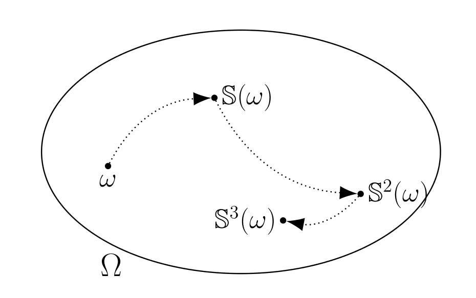
Fig. 1.1 The evolution of a sample point \(\omega\) induced by successive applications of the transformation \(\mathbb{S}\). The oval shaped region is the collection \(\Omega\) of all sample points.

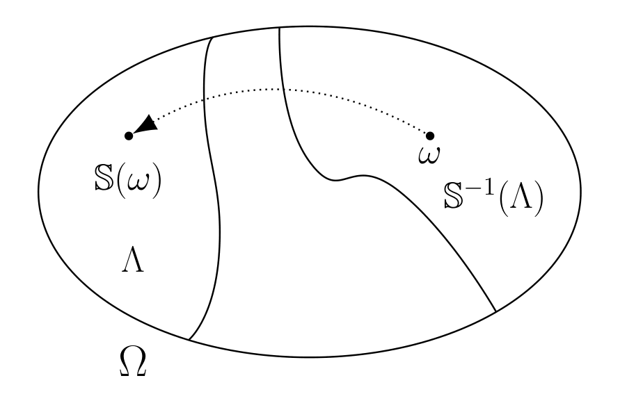
Fig. 1.2 An inverse image \(\mathbb{S}^{-1}(\Lambda)\) of an event \(\Lambda\) is itself an event; \(\omega \in \mathbb{S}^{-1}(\Lambda)\) implies that \(\mathbb{S}(\omega)\in \Lambda\).

We use two objects.[2]

The first is a (measurable) transformation \({\mathbb S}: \Omega \rightarrow \Omega\) that describes the evolution of a sample point \(\omega\). See Fig. 1.1. Transformation \({\mathbb S}\) has the property that for any event \(\Lambda \in {\mathfrak F}\),

\[{\mathbb S}^{-1}(\Lambda) = \{\omega \in \Omega : {\mathbb S}(\omega) \in \Lambda\}\]

is an event in \({\mathfrak F}\), as depicted in Fig. 1.2. The second object is an \(n\)-dimensional vector \(X(\omega)\) that describes how observations depend on sample point \(\omega\).

We construct a stochastic process \(\{ X_t : t = 0,1,... \}\) via the formula:

\[X_t(\omega) = X[{\mathbb S}^t(\omega)]\]

or

\[X_t = X \circ {\mathbb S}^t,\]

where we interpret \({\mathbb S}^0\) as the identity mapping asserting that \(\omega_0 = \omega\).

Because a known function \({\mathbb S}\) maps a sample point \(\omega \in \Omega\) today into a sample point \({\mathbb S}(\omega) \in \Omega\) tomorrow, the evolution of sample points is deterministic: \(\omega_{t+j}\) for all \(j \geq 1\) can be predicted perfectly if we know \({\mathbb S}\) and \(\omega_t\). But we do not observe \(\omega_t\) at any \(t\). Instead, we observe an \((n \times 1)\) vector \(X(\omega)\) that contains incomplete information about \(\omega\). We assign probabilities \(Pr\) to collections of sample points \(\omega\) called events, then use the functions \({\mathbb S}\) and \(X\) to induce a joint probability distribution over sequences of \(X\)’s. The resulting stochastic process \(\{ X_t : t=0,1,2,...\}\) is a sequence of \(n\)-dimensional random vectors.

This way of constructing a stochastic process might seem restrictive; but actually, it is more general than the canonical construction presented above.

Example 1.1

Consider again our canonical construction 1.1. Recall that the set of sample points \(\Omega\) is the collection of infinite sequences of elements of \({\mathbf r}_t \in {\mathbb R}^n\) so that \(\omega = ({\mathbf r}_0, {\mathbf r}_1, ... )\). For this example, \({\mathbb S}(\omega) = ({\mathbf r}_1,{\mathbf r}_2, ...)\). This choice of \({\mathbb S}\) is called the shift transformation. Notice that the time \(t\) iterate is

\[{\mathbb S}^t(\omega) = ({\mathbf r}_t, {\mathbf r}_{t+1}, ... )\]

Let the measurement function be: \(X(\omega) = {\mathbf r}_0\) so that

\[X_t(\omega) = X\left[ {\mathbb S}^t (\omega)\right] = {\mathbf r}_t\]

as posited in construction 1.1.

1.4. Stationary Stochastic Processes

We start with a probabilistic notion of invariance. We call a stochastic process stationary if for any finite integer \(\ell\), the joint probability distribution induced by the composite random vector \(\left[{X_{t}}',{X_{t+1}}',...,{X_{t+\ell}}'\right]'\) is the same for all \(t \ge 0\).[3] This notion of stationarity can be thought of as a stochastic version of a steady state of a dynamical system.

We now use the objects \(({\mathbb S}, X)\) to build a stationary stochastic process by restricting construction 1.1.
Consider the set \( \{ \omega \in \Omega : X(\omega) \in \mathfrak{b} \} \doteq \Lambda\) and its successors

\[\begin{split}\begin{align*} \{ \omega \in \Omega : X_1 (\omega) \in \mathfrak{b} \} & = \{ \omega \in \Omega : X\left[ {\mathbb S} (\omega) \right] \in \mathfrak{b} \} = {\mathbb S}^{-1}(\Lambda) \\ \{ \omega \in \Omega : X_t (\omega) \in \mathfrak{b} \} & = \{ \omega \in \Omega : X\left[ {\mathbb S}^t (\omega) \right] \in \mathfrak{b} \} = {\mathbb S}^{-t}(\Lambda) . \end{align*}\end{split}\]

Evidently, if \(Pr(\Lambda) = Pr[{\mathbb S}^{-1}(\Lambda)]\) for all \(\Lambda \in {\mathfrak F}\), then the probability distribution induced by \(X_{t}\) equals the probability distribution of \(X\) for all \(t\). This fact motivates the following definition and proposition.

Definition 1.3

The pair \(({\mathbb S}, Pr)\) is said to be measure-preserving if

\[Pr ( \Lambda ) = Pr \{ {\mathbb S}^{-1}(\Lambda) \}\]

for all \(\Lambda \in {\mathfrak F}\).

Theorem 1.1

When \((\mathbb{S}, Pr)\) is measure-preserving, probability distributions induced by the random vectors \(X_t\) are identical for all \(t \ge 0\).

The measure preserving property restricts the probability measure \(Pr\) for a given transformation \(\mathbb{S}\). Some probability measures \(Pr\) used in conjunction with \(\mathbb{S}\) will be measure preserving and others not, a fact that will play an important role at several places below.

Suppose that \((\mathbb{S}, Pr)\) is measure preserving relative to probability measure \(Pr\). Given \(X\) and an integer \(\ell > 1\), form a vector

\[\begin{split}X^{[\ell]} (\omega) \doteq \begin{bmatrix} X_0(\omega) \\ X_1(\omega) \\ ... \\ X_\ell(\omega) \end{bmatrix}.\end{split}\]

We can apply Theorem 1.1 to \(X^{[\ell]}\) to conclude that the joint distribution function of \((X_{t}, X_{t+1}, ..., X_{t+\ell})\) is independent of \(t\) for \(t = 0,1,\ldots\). That this property holds for any choice of \(\ell\) implying that the stochastic process \(\{ X_t : t=1,2, ...\}\) is stationary. Moreover, \(f\left( X^\ell\right)\) where \(f\) is a Borel measurable function from \(\mathbb{R}^{n(\ell+1)}\) into \(\mathbb{R}\) is also a valid measurement function. Such \(f\)’s include indicator functions of interesting events defined in terms of \(X^\ell\).

For a given \(\mathbb{S}\), we now present examples that illustrate how to construct a probability measure \(Pr\) that makes \(\mathbb{S}\) measure preserving and thereby brings stationarity.

Example 1.2

Suppose that \(\Omega\) contains two points, \(\Omega = \{\omega_1, \omega_2 \}\). Consider a transformation \(\mathbb{S}\) that maps \(\omega_1\) into \(\omega_2\) and \(\omega_2\) into \(\omega_1\): \(\mathbb{S}(\omega_1 ) = \omega_2\) and \(\mathbb{S}( \omega_2 ) = \omega_1\). Since \(\mathbb{S}^{-1}(\{\omega_2\}) = \{\omega_1\}\) and \(\mathbb{S}^{-1}(\{\omega_1\}) = \{\omega_2 \}\), for \(\mathbb{S}\) to be measure preserving, we must have \(Pr(\{\omega_1\}) = Pr(\{\omega_2\}) = 1/2\).

Example 1.3

Suppose that \(\Omega\) contains two points, \(\Omega = \{\omega_1, \omega_2\}\) and that \({\mathbb S}(\omega_1) = \omega_1 \) and \({\mathbb S}( \omega_2 ) = \omega_2\). Since \({\mathbb S}^{-1}(\{\omega_2\}) = \{\omega_2\}\) and \({\mathbb S}^{-1}(\{\omega_1\}) = \{\omega_1\}\), \({\mathbb S}\) is measure preserving for any \(Pr\) that satisfies \(Pr(\{\omega_1\}) \geq 0\) and \( Pr(\{\omega_2\}) = 1 -Pr(\{\omega_1\}) \).

The next example illustrates how to represent an i.i.d. sequence of zeros and ones in terms of an \(\Omega, Pr\) and an \({\mathbb S}\).

Example 1.4

Suppose that \(\Omega = [0,1)\) and that \(Pr\) is the uniform measure on \([0,1)\). Let

\[\begin{align*} {\mathbb S}(\omega) & = \left\{ \begin{matrix} 2 \omega & if \ \omega \in [0,1/2) \cr 2 \omega - 1 & if \ \omega \in [1/2,1), \end{matrix} \right\}. \cr X(\omega) & = \left\{ \begin{matrix} 1 & if \ \omega \in [0,1/2) \cr 0 & if \ \omega \in [1/2,1) .\end{matrix} \right\}. \end{align*}\]

Calculate \(Pr \left\{ X_1 = 1 \vert X_0 = 1 \right\} = Pr \left\{ X_1 = 1\vert X_0 = 0 \right\} = Pr \left\{ X_1 = 1 \right\} = 1/2\) and \(Pr \left\{ X_1 = 0 \vert X_0 = 1 \right\} = Pr \left\{ X_1 = 0\vert X_0 = 0 \right\} = Pr \left\{ X_1 = 0 \right\} = 1/2\). So \(X_1\) is statistically independent of \(X_0\). By extending these calculations, it can be verified that \(\{ X_t : t=0,1,...\}\) is a sequence of independent random variables.[4] We can alter \(Pr\) to obtain other stationary distributions. For instance, suppose that \(Pr\{ \frac 1 3\} = Pr \{ \frac 2 3 \} = .5\). Then the process \(\{ X_t : t=0,1,...\}\) alternates in a deterministic fashion between zero and one. This provides a version of Example 1.2 in which \(\omega_1 = \frac{1}{3}\) and \(\omega_2 = \frac{2}{3}\).

1.5. Invariant Events and Conditional Expectations

In this section, we present a Law of Large Numbers that asserts that time series averages converge when \({\mathbb S}\) is measure-preserving relative to \(Pr\).

1.5.1. Invariant events

We use the concept of an invariant event to understand how limit points of time series averages relate to a conditional mathematical expectation.

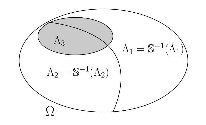
Fig. 1.3 Two invariant events \(\Lambda_1\) and \(\Lambda_2\) and an event \(\Lambda_3\) that is not invariant.

Definition 1.4

An event \(\Lambda\) is invariant if \(\Lambda = {\mathbb S}^{-1}(\Lambda)\).

Fig. 1.3 illustrates two invariant events in a space \(\Omega\). Notice that if \(\Lambda\) is an invariant event and \(\omega \in \Lambda\), then \({\mathbb S}^t(\omega) \in \Lambda\) for \(t = 0,1,...,\infty\).

Let \({\mathfrak I}\) denote the collection of invariant events. The entire space \(\Omega\) and the null set \(\varnothing\) are both invariant events. Like \({\mathfrak F}\), the collection of invariant events \({\mathfrak I}\) is a sigma algebra.

1.5.2. Conditional expectation

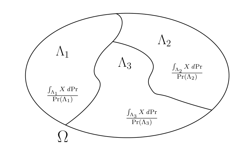
Fig. 1.4 A conditional expectation \(E(X | {\mathfrak I})\) is constant for \(\omega \in \Lambda_j = {\mathbb S}^{-1}(\Lambda_j)\).

We want to construct a random vector \(E(X|{\mathfrak I})\) called the “mathematical expectation of \(X\) conditional on the collection \({\mathfrak I}\) of invariant events”. We begin with a situation in which a conditional expectation is a discrete random vector as occurs when invariant events are unions of sets \(\Lambda_j\) belonging to a countable partition of \(\Omega\) (together with the empty set). Later we’ll extend the definition beyond this special setting.

A countable partition consists of a countable collection of nonempty events \(\Lambda_j\) such that \(\Lambda_j \cap \Lambda_k = \varnothing\) for \(j \ne k\) and such that the union of all \(\Lambda_j\) is \(\Omega\). Assume that each set \(\Lambda_j\) in the partition is itself an invariant event. Define the mathematical expectation conditioned on event \(\Lambda_j\) as

\[\frac {\int_{\Lambda_j} X dPr} {Pr(\Lambda_j)}\]

when \(\omega \in \Lambda_j\). To extend the definition of conditional expectation to all of \({\mathfrak I}\), take

\[E(X|{\mathfrak I} )(\omega) = \frac {\int_{\Lambda_j} X dPr} {Pr(\Lambda_j)} \ \ \textrm{if} \ \ \omega \in \Lambda_j.\]

Thus, the conditional expectation \(E(X | {\mathfrak I})\) is constant for \(\omega \in \Lambda_j\) but varies across \(\Lambda_j\)’s. Fig. 1.4 illustrates this characterization for a finite partition.

1.5.3. Least Squares

Now let \(X\) be a random vector with finite second moments \( E XX' = \int X(\omega) X(\omega)' d Pr(\omega)\). When a random vector \(X\) has finite second moments, a conditional expectation is a least squares projection. Let \(Z\) be an \(n\)-dimensional measurement function that is time-invariant and so satisfies

\[Z_t(\omega) = Z[{\mathbb S}^t(\omega)] = Z(\omega) .\]

Let \({\mathcal Z}\) denote the collection of all such time-invariant random vectors. In the special case in which the invariant events can be constructed from a finite partition, \(Z\) can vary across sets \(\Lambda_j\) but must remain constant within \(\Lambda_j\).[5] Consider the least squares problem

(1.2)\[min_{Z \in {\mathcal Z}} E[|X - Z|^2] .\]

Denote the minimizer in problem (1.2) by \({\tilde X} = E(X \vert {\mathfrak I})\). Necessary conditions for the least squares minimizer \(\widetilde X \in {\mathcal Z}\) imply that

\[E[(X - {\widetilde X})Z'] = 0\]

for \(Z\) in \({\mathcal Z}\) so that each entry of the vector \(X-{\widetilde X}\) of regression errors is orthogonal to every vector \(Z\) in \({\mathcal Z}\).

A measure-theoretic approach constructs a conditional expectation by extending the orthogonality property of least squares. Provided that \(E|X| < \infty\), \(E(X|{\mathfrak I})(\omega)\) is the essentially unique random vector that, for any invariant event \(\Lambda\), satisfies

\[E([ X - E(X \vert {\mathfrak I})] \textbf{1}_\Lambda ) = 0,\]

where \(\textbf{1}_\Lambda\) is the indicator function that is equal to one on the set \(\Lambda\) and zero otherwise.

1.6. Law of Large Numbers

An elementary Law of Large Numbers asserts that the limit of an average over time of a sequence of independent and identically distributed random vectors equals the unconditional expectation of the random vector. We want a more general Law of Large Numbers that applies to averages over time of sequences of observations that are intertemporally dependent. To do this, we use a notion of probabilistic invariance that is expressed in terms of the measure-preserving restriction and that implies a Law of Large Numbers applicable to stochastic processes.

The following theorem asserts two senses in which averages of intertemporally dependent processes converge to mathematical expectations conditioned on invariant events.

Theorem 1.2

(Birkhoff) Suppose that \(\mathbb{S}\) is measure preserving relative to the probability space \((\Omega, \mathfrak{F}, Pr)\).[6]

1. For any \(X\) such that \(E|X| < \infty\),

\[\frac{1}{N} \sum_{t=1}^N X_t(\omega) \rightarrow E(X|\mathfrak{I})(\omega)\]

with probability one;

2. For any \(X(\omega)\) such that \(E|X(\omega)|^2 < \infty\),

\[E \left[ \left| \frac{1}{N} \sum_{t=1}^N X_t - E(X|\mathfrak{I}) \right|^2 \right] \rightarrow 0.\]

Part 1) asserts almost-sure convergence; part 2) asserts mean-square convergence.

We have ample flexibility to specify a measurement function \(\phi \left( X^\ell\right),\) where \(\phi\) is a Borel measurable function from \(\mathbb{R}^{n(\ell+1)}\) into \(\mathbb{R}\). In particular, an indicator functions for event \(\Lambda = \{X^\ell \in \mathfrak{b} \}\) can be used as a measurement function where:

\[\begin{split}{\bf 1}_\Lambda(\omega) = \begin{cases} 1 & \text{if} \ \omega \in \Lambda \\ 0 & \text{if} \ \omega \notin \Lambda. \end{cases}\end{split}\]

The Law of Large Numbers applies to limits of

\[\frac{1}{N} \sum_{t=1}^N \phi\left[ X_t^\ell \right]\]

for alternative \(\phi\)’s, so choosing \(\phi\)’s to be indicator functions shows how the Law of Large Numbers uncovers event probabilities of interest.

Definition 1.5

A transformation \(\mathbb{S}\) that is measure-preserving relative to \(Pr\) is said to be ergodic under probability measure \(Pr\) if all invariant events have probability zero or one.

Thus, when a transformation \(\mathbb{S}\) is ergodic under measure \(Pr\), the invariant events have either the same probability measure as the entire sample space \(\Omega\) (whose probability measure is one), or the same probability measure as the empty set \(\varnothing\) (whose probability measure is zero).

Proposition 1.1

Suppose that the measure preserving transformation \(\mathbb{S}\) is ergodic under measure \(Pr\). Then \(E(X|\mathfrak{I}) = E(X)\).

Theorem 1.2 describes conditions for convergence in the general case that \(\mathbb{S}\) is measure preserving under \(Pr\), but in which \(\mathbb{S}\) is not necessarily ergodic under \(Pr\). Proposition 1.1 describes a situation in which probabilities assigned to invariant events are degenerate in the sense that all invariant events have the same probability as either \(\Omega\) (probability one) or the null set (probability zero). When \(\mathbb{S}\) is ergodic under measure \(Pr\), limit points of time series averages equal corresponding unconditional expectations, an outcome we can call a standard Law of Large Numbers. When \(\mathbb{S}\) is not ergodic under \(Pr\), limit points of time series averages equal expectations conditioned on invariant events.

The following examples remind us how ergodicity restricts \(\mathbb{S}\) and \(Pr\).

Example 1.5

Consider Example 1.2 again.
\(\Omega\) contains two points and \(\mathbb{S}\) maps \(\omega_1\) into \(\omega_2\) and \(\omega_2\) into \(\omega_1\): \(\mathbb{S}(\omega_1) = \omega_2\) and \(\mathbb{S}(\omega_2) = \omega_1\). Suppose that the measurement vector is

\[\begin{split}X(\omega) = \left\{ \begin{matrix} 1 & \ {\textrm{if}} \ \omega = \omega_1 \\ 0 & \ \textrm{if} \ \omega = \omega_2 . \end{matrix} \right.\end{split}\]

Then it follows directly from the specification of \(\mathbb{S}\) that

\[{\frac 1 N} \sum_{t=1}^N X_t(\omega) \rightarrow {\frac 1 2}\]

for both values of \(\omega\). The limit point is the average across sample points.

Example 1.6

Return to Example 1.3. \(\Omega\) contains two points, \(\Omega = \{\omega_1, \omega_2\}\) and that \({\mathbb S}(\omega_1) = \omega_1 \) and \({\mathbb S}( \omega_2 ) = \omega_2\). \(X_t(\omega)= X(\omega)\) so that the sequence is time invariant and equal to its time-series average. A time-series average of \(X_t(\omega)\) equals the average across sample points only when \(Pr\) assigns probability \(1\) to either \(\omega_1\) or \(\omega_2\).

1.7. Limiting Empirical Measures

Given a triple \((\Omega, {\mathfrak F}, Pr)\) and a measure-preserving transformation \({\mathbb S}\), we can use Theorem 1.2 to construct limiting empirical measures on \({\mathfrak F}\). To start, we will analyze a setting with a countable partition of \(\Omega\) consisting of invariant events \(\{ \Lambda_j : j=1,2,... \}\), each of which has strictly positive probability under \(Pr\). We consider a more general setting later. Given an event \(\Lambda\) in \({\mathfrak F}\) and for almost all \(\omega \in \Lambda_j\), define the limiting empirical measure \(Qr_j\) as

(1.3)\[Qr_j(\Lambda)(\omega) = \lim_{N \rightarrow \infty} {\frac 1 N} \sum_{t=1}^N {\bf 1}_\Lambda\left[ {\mathbb S}^t(\omega) \right] = {\frac {Pr(\Lambda \cap \Lambda_j)} { Pr(\Lambda_j)}.}\]

Thus, when \(\omega \in \Lambda_j\), \(Qr_j(\Lambda)\) is the fraction of time \({\mathbb S}^t(\omega) \in \Lambda\) in very long samples. If we hold \(\Lambda_j\) fixed and let \(\Lambda\) be an arbitrary event in \({\mathfrak F}\), we can treat \(Qr_j\) as a probability measure on \((\Omega, {\mathfrak F})\). By doing this for each \(\Lambda_j, j = 1, 2, \ldots\), we can construct a countable set of probability measures \(\{Qr_j\}_{j=1}^\infty\). These comprise the set of all measures that can be recovered by applying the Law of Large Numbers. If nature draws an \(\omega \in \Lambda_j\), then measure \(Qr_j\) describes outcomes.

So far, we started with a probability measure \(Pr\) and then constructed the set of possible limiting empirical measures \(Qr_j\)’s. We now reverse the direction of the logic by starting with probability measures \(Qr_j\) and then finding measures \(Pr\) that are consistent with them. We do this because \(Qr_j\)’s are the only measures that long time series can disclose through the Law of Large Numbers: each \(Qr_j\) defined by (1.3) uses the Law of Large Numbers to assign probabilities to events \(\Lambda \in {\mathfrak F}\). However, because

\[ Qr_j(\Lambda) = Pr( \Lambda \mid \Lambda_j ) = {\frac {Pr(\Lambda \cap \Lambda_j)} { Pr(\Lambda_j)} } \textrm{ for } j = 1, 2, \ldots , \]

are conditional probabilities, such \(Qr_j\)’s are silent about the probabilities \(Pr(\Lambda_j)\) of the underlying invariant events \(\Lambda_j\). There are multiple ways to assign probabilities \(Pr\) that imply identical probabilities conditioned on invariant events.

Because \(Qr_j\) is all that can ever be learned by “letting the data speak”, we regard each probability measure \(Qr_j\) as a statistical model.[7]

Proposition 1.2

A statistical model is a probability measure that a Law of Large Numbers can disclose.

Probability measure \(Qr_j\) describes a statistical model associated with invariant set \(\Lambda_j\).

Remark 1.1

For each \(j\), \({\mathbb S}\) is measure-preserving and ergodic on \((\Omega, {\mathfrak F}, Qr_j)\).
The second equality of definition (1.3) assures ergodicity by assigning probability one to the event \(\Lambda_j\).

Relation (1.3) implies that probability \(Pr\) connects to probabilities \(Qr_j\) by

(1.4)\[Pr(\Lambda) = \sum_j Qr_j(\Lambda) Pr(\Lambda_j).\]

While decomposition (1.4) follows from definitions of the elementary objects that comprise a stochastic process and is “just mathematics”, it is interesting because it tells how to construct alternative probability measures \(Pr\) for which \({\mathbb S}\) is measure preserving. Because long data series disclose probabilities conditioned on invariant events to be \(Qr_j\), to respect evidence from long time series we must hold the \(Qr_j\)’s fixed, but we can freely assign probabilities \(Pr\) to invariant events \(\Lambda_j\). In this way, we can create a family of probability measures for which \({\mathbb S}\) is measure preserving.

1.8. Ergodic Decomposition

Up to now, we have represented invariant events with a countable partition. Dynkin [1978] deduced a more general version of decomposition (1.4) without assuming a countable partition. Thus, start with a pair \((\Omega, \mathfrak{F})\). Also, assume that there is a metric on \(\Omega\) and that \(\Omega\) is separable. We also assume that \(\mathfrak{F}\) is the collection of Borel sets (the smallest sigma algebra containing the open sets). Given \((\Omega, \mathfrak{F})\), take a (measurable) transformation \(\mathbb{S}\) and consider the set \(\mathcal{P}\) of probability measures \(Pr\) for which \(\mathbb{S}\) is measure-preserving. For some of these probability measures, \(\mathbb{S}\) is ergodic, but for others, it is not. Let \(\mathcal{Q}\) denote the set of probability measures for which \(\mathbb{S}\) is ergodic. Under a nondegenerate convex combination of two probability measures in \(\mathcal{Q}\), \(\mathbb{S}\) is measure-preserving but not ergodic. Dynkin [1978] constructed limiting empirical measures \(Qr\) on \(\mathcal{Q}\) and justified the following representation of the set \(\mathcal{P}\) of probability measures \(Pr\).

Proposition 1.3

For each probability measure \(\widetilde{Pr}\) in \({\mathcal P}\), there is a unique probability measure \(\pi\) over \({\mathcal Q}\) such that

(1.5)\[\widetilde{Pr}(\Lambda) = \int_{{\mathcal Q}} Qr(\Lambda) \pi(dQr)\]

for all \(\Lambda \in {\mathfrak F}\).[8]

Proposition 1.3 generalizes representation (1.4). It asserts a sense in which the set \({\mathcal P}\) of probabilities for which \({\mathbb S}\) is measure-preserving is convex. Extremal points of this set are in the smaller set \({\mathcal Q}\) of probability measures for which the transformation \({\mathbb S}\) is ergodic. Representation (1.5) shows that by forming “mixtures” (i.e., weighted averages or convex combinations) of probability measures under which \({\mathbb S}\) is ergodic, we can represent all probability specifications for which \({\mathbb S}\) is measure-preserving.

To add another perspective, a collection of invariant events \({\mathfrak I}\) is associated with a transformation \({\mathbb S}\). There exists a common conditional expectation operator \( {\mathbb J} \equiv E(\cdot |{\mathfrak I})\) that assigns mathematical expectations to bounded measurable functions (mapping \(\Omega\) into \({\mathbb R}\)) conditioned on the set of invariant events \({\mathfrak I}\). The conditional expectation operator \({\mathbb J} \) characterizes limit points of time series averages of indicator functions of events of interest as well as other random vectors. Alternative probability measures \({Pr}\) assign different probabilities to the invariant events.

1.9. Risk and Uncertainty

An applied researcher typically does not know which statistical model generated the data. This situation leads us to specifications of \(\mathbb{S}\) that are consistent with a family \(\mathcal{P}\) of probability models under which \(\mathbb{S}\) is measure preserving and a stochastic process is stationary. Representation (1.5) describes uncertainty about statistical models with a probability distribution \(\pi\) over the set of statistical models \(\mathcal{Q}\).

For a Bayesian, \(\pi\) is a subjective prior probability distribution that pins down a convex combination of “statistical models.”[9] A Bayesian expresses trust in that convex combination of statistical models used to construct a complete probability measure over outcomes[10] and uses it to compute expected utility. A Bayesian decision theory axiomatized by Savage makes no distinction between how decision makers respond to the probabilities described by the component statistical models and the \(\pi\) probabilities that he uses to mix them. All that matters to a Bayesian decision maker is the complete probability distribution over outcomes, not how it is attained as a \(\pi\)-mixture of component statistical models.

Some decision and control theorists challenge the complete confidence in a single prior probability assumed in a Bayesian approach.[11] They want to distinguish ‘ambiguity’, meaning not being able confidently to assign \(\pi\), from ‘risk’, meaning prospective outcomes with probabilities reliably described by a statistical model. They imagine decision makers who want to evaluate decisions under alternative \(\pi\)’s.[12] We explore these ideas in later chapters.

An important implication of the Law of Large Numbers is that for a given initial \(\pi\), using Bayes’ rule to update the \(\pi\) probabilities as data arrive will eventually concentrate posterior probability on the statistical model that generates the data. Even when a decision maker entertains a family of \(\pi\)’s, the updated probabilities conditioned on the data may still concentrate on the statistical model that generates the data.

1.10. Inventing an Infinite Past

When \(Pr\) is measure preserving and the process \(\{ X_t : t = 0,1,... \}\) is stationary, it can be useful to invent an infinite past. To accomplish this, we reason in terms of the (measurable) transformation \({\mathbb S} : \Omega \rightarrow \Omega\) that describes the evolution of a sample point \(\omega\). Until now we have assumed that \({\mathbb S}\) has the property that for any event \(\Lambda \in {\mathfrak F}\),

\[{\mathbb S}^{-1}(\Lambda) = \{\omega \in \Omega : {\mathbb S}(\omega) \in \Lambda\}\]

is an event in \({\mathfrak F}\). In Section Stationary Increments, we want more. To prepare the way for that chapter, in this section we shall also assume that \({\mathbb S}\) is one-to-one and has the property that for any event \(\Lambda \in {\mathfrak F}\),

(1.6)\[{\mathbb S}(\Lambda) = \{\omega \in \Omega : {\mathbb S}^{-1} (\omega) \in \Lambda\} \in {\mathfrak F} .\]

Because

\[X_t(\omega) = X[{\mathbb S}^t(\omega)] = X_t = X \circ {\mathbb S}^t\]

is well defined for negative values of \(t\), restrictions (1.6) allow us to construct a ``two-sided’’ process that has both an infinite past and an infinite future.

Let \({\mathfrak A}\) be a subsigma algebra of \({\mathfrak F}\), and let

(1.7)\[{\mathfrak A}_t = \left\{ \Lambda_t \in {\mathfrak F} : \Lambda_t = \{ \omega \in \Omega : {\mathbb S}^t(\omega) \in \Lambda \} \textrm{ for some } \Lambda \in {\mathfrak F} \right\}.\]

We assume that \(\{ {\mathfrak A}_t : - \infty < t < + \infty \}\) is a nondecreasing {\em filtration}. If the original measurement function \(X\) is \({\mathfrak A}\)-measurable, then \(X_t\) is \({\mathfrak A}_t\)-measurable. Furthermore, \(X_{t-j}\) is in \({\mathfrak A}_t\) for all \(j \ge 0\). The set \({\mathfrak A}_t\) depicts information available at date \(t\), including past information. Invariant events in \({\mathfrak I}\) are contained in \({\mathfrak A}_t\) for all \(t\).

We construct the following moving-average representation of a scalar process \(\{X_t\}\) in terms of an infinite history of shocks.

Example 1.7

(Moving average) Suppose that \(\{W_t : -\infty < t < \infty \}\) is a vector stationary process for which[13]

\[E\left( W_{t+1} \vert {\mathfrak A}_t \right) = 0\]

and that

\[E\left( W_t{W_t}' \vert {\mathfrak I} \right) = I\]

for all \(-\infty < t < +\infty\).
Use a sequence of vectors \(\{\alpha_j\}_{j=0}^\infty \) to construct

(1.8)\[X_t = \sum_{j=0}^\infty \alpha_j \cdot W_{t-j}\]

where

(1.9)\[\sum_{j=0}^\infty \vert \alpha_j \vert^2 < \infty .\]

Restriction (1.9) implies that \(X_t\) is well defined as a mean square limit. \(X_t\) is constructed from the infinite past \(\{ W_{t-j} : 0 \leq j < \infty \}\). The process \(\{X_t : - \infty < t < \infty \}\) is stationary and is often called an infinite-order moving average process. The sequence \(\{ \alpha_j : j=0,1,... \}\) can depend on the invariant events.

Remark 1.2

Almost a century ago, both Slutsky [1927] and Yule [1927] used probability models to analyze economic time series. Their models implied moving-average representations like the one in Example 1.7. Their idea was to see economic time series as responding linearly to current and past independent and identically distributed impulses or shocks. In distinct contributions, they showed how such models generate recurrent but aperiodic fluctuations that resemble business cycles and longer-term cycles as well. Yule [1927] and Slutsky [1927] came from different backgrounds and brought different perspectives. Yule [1927] was an eminent statistician who, among other important contributions, managed “effectively to invent modern time series analysis” in the words of Stigler [1986]. Yule constructed and estimated what we would now call a second-order autoregression and applied it to study sunspots. Yule’s estimates implied \(\alpha_j\) coefficients showed damped oscillations at the same periodicity as sunspots. In Russia in the 1920s, Slutsky [1927] wrote a seminal paper in Russian motivated by his interest in business cycles. Only later was an English version of his paper published Econometrica. Even before that, it was already on the radar screen of economists including Ragnar Frisch. Indeed, Frisch was keenly aware of both Slutsky [1927] and Yule [1927] and generously acknowledged both of them in his seminal paper Frisch [1933] on the impulse and propagation problem. Building on insights of Slutsky [1927] and Yule [1927], Frisch [1933] pioneered impulse response functions. His ambition was to provide explicit economic interpretations for how shocks alter economic time series both now and later.[14]

1.11. Summary

For a fixed \(\mathbb{S}\) there are often many possible probabilities \(Pr\) that are measure preserving. A subset of these are ergodic. These ergodic probabilities can serve as building blocks for the other measure preserving probabilities. Thus, each measure preserving \(Pr\) can be expressed as a weighted average of the ergodic probabilities. We call the ergodic probabilities statistical models. The Law of Large Numbers applies to each of the ergodic building blocks with limit points that are unconditional expectations. As embodied in (1.4) and its generalization (1.5), this decomposition interests both frequentist and Bayesian statisticians.

---

[1]

This essentially follows from the Kolomorov Extension Theorem or from Theorem 2.26 of Breiman [1968].

[2]

Breiman [1968] is a good reference for these.

[3]

Sometimes this property is called `strict stationarity’ to distinguish it from weaker notions that require only that some moments of joint distributions be independent of time. What is variously called wide-sense or second-order or covariance stationarity requires only that first and second moments of joint distributions are independent of calendar time.

[4]

This example is from Breiman [1968][p. 108].

[5]

More generally, \(Z\) must be measurable with respect to \({\mathfrak I}\).

[6]

See Breiman [1968] chapter 6 for extended discussions and proofs.

[7]

Marschak [1953], Hurwicz [1962], Lucas [1976], and Sargent [1981] distinguished between structural econometric models and what we call statistical models. Structural econometric models are designed to forecast outcomes of hypothetical experiments that freeze some components of an economic environment and change others. A structural model accepts experiments that alter statistical models.

[8]

Krylov and Bogolioubov [1937] provide an early statement of this result. Dynkin [1978] provides a more general formulation that nests this and other closely related results. His analysis includes a formalization of integration over the probability measures in \({\mathcal Q}\). Dynkin [1978] uses the resulting representation to draw connections between collections of invariant events and sets of sufficient statistics.

[9]

This subsection is motivated in part by the intriguing discussions of von Plato [1982] and Cerreia-Vioglio et al. [2013].

[10]

Here ‘complete’ can be taken to be synonymous with ‘not conditioning on invariant events’.

[11]

For example, see Hansen and Sargent [2008].

[12]

This gives one way to formalize ideas of Knight [1921], who sought to distinguish risk from broader notions of uncertainty.

[13]

An i.i.d.~sequence is just one example of such a \(\{W_t : -\infty < t < \infty \}\) process.

[14]

Sims [1980] and others advanced this idea by developing tractable multivariate time series methods and striving to isolate interpretable shocks in multivariate settings.