6. Hidden Markov Models

6.1. Sufficient Statistics as States

This chapter presents Hidden Markov Models that start from a joint probability distribution consisting of a Markov process and a vector of noise-ridden signals about functions of the Markov state. Histories of signals are observed but the Markov state vector is not. Statistical learning about the Markov state proceeds by constructing a sequence of probability distributions of the Markov state conditional on histories of signals. Recursive representations of these conditional distributions form auxiliary Markov processes that summarize all information about the hidden state vector contained in histories of signals. A state vector in this auxiliary Markov process is a set of sufficient statistics for the probability distribution of the hidden Markov state conditional on the history of signals. We can construct this auxiliary Markov process of sufficient statistics sequentially.

We present four examples of Hidden Markov Models that are used to learn about

1. A continuously distributed hidden state vector in a linear state-space system

2. A discrete hidden state vector

3. Multiple VAR regimes

4. Unknown parameters cast as hidden invariant states

6.2. Kalman Filter and Smoother

We assume that a Markov state vector \(X_t\) and a vector \(Z_{t+1}\) of observations are governed by a linear state space system

(6.1)\[\begin{split}\begin{align} X_{t+1} & = {\mathbb A} X_t + {\mathbb B} W_{t+1} \\ Z_{t+1} & = {\mathbb H} + {\mathbb D} X_t + {\mathbb F} W_{t+1}, \end{align}\end{split}\]

where the matrix \({\mathbb F}{\mathbb F}' \) is nonsingular, \(X_t\) has dimension \(n\), \(Z_{t+1}\) has dimension \(m\) and is a signal observed at \(t+1\), \(W_{t+1}\) has dimension \(k\) and is a standard normally distributed random vector that is independent of \(X_t\), of \(Z^t = [Z_t, \ldots , Z_1]\), and of \(X_0.\) The initial state vector \(X_0 \sim Q_0\), where \(Q_0\) is a normal distribution with mean \(\overline X_0\) and covariance matrix \(\Sigma_0\).[1] To include the ability to represent an unknown fixed parameter as an invariant state associated with a unit eigenvalue in \(A\), we allow \(A\) not to be a stable matrix.

Although \(\{(X_t, Z_t), t=0, 1, 2, \ldots \}\) is Markov, \(\{ Z_{t}, t=0, 1, 2, \ldots \}\) is not.[2] We want to construct an affiliated Markov process whose date \(t\) state is \(Q_t\), defined to be the probability distribution of the time \(t\) Markov state \(X_t\) conditional on history \(Z^t =Z_t, \ldots , Z_1\) and \(Q_0\). The distribution \(Q_t\) summarizes information about \(X_t\) that is contained in the history \(Z^t\) and \(Q_0\). We sometimes use \(Q_t\) to indicate conditioning information that is “random” in the sense that it is constructed from a history of observable random vectors. Because the distribution \(Q_t\) is multivariate normal, it suffices to keep track only of the mean vector \({\overline X}_t\) and covariance matrix \(\Sigma_t\) of \(X_t\) conditioned on \(Q_0\) and \(Z^{t}\): \({\overline X}_t\) and \(\Sigma_t\) are sufficient statistics for the probability distribution of \(X_t\) conditional on the history \(Z^{t}\) and \(Q_0\). Conditioning on \(Q_t\) is equivalent to conditioning on these sufficient statistics.

We can map sufficient statistics \((\overline X_{j-1}, \Sigma_{j-1})\) for \(Q_{j-1}\) into sufficient statistics \((\overline X_j, \Sigma_j\)) for \(Q_j\) by applying formulas for means and covariances of a conditional distribution associated with a multivariate normal distribution. This generates a recursion that maps \(Q_{j-1}\) and \(Z_{j}\) into \(Q_j\). It enables us to construct \(\{Q_t\}\) sequentially. Thus, consider the following three step process.

1. Express the joint distribution of \(X_{t+1}, Z_{t+1}\) conditional on \(X_t\) as

\[\begin{split}\begin{bmatrix} X_{t+1} \\ Z_{t+1} \end{bmatrix} \sim \mathcal{N}\left(\begin{bmatrix} 0 \\ {\mathbb H} \end{bmatrix} + \begin{bmatrix} {\mathbb A} \\ {\mathbb D} \end{bmatrix} X_t, \begin{bmatrix} {\mathbb B} \\ {\mathbb F} \end{bmatrix} \begin{bmatrix} {\mathbb B}' & {\mathbb F}' \end{bmatrix} \right). \end{split}\]

2. Suppose that the distribution \(Q_t\) of \(X_t\) conditioned on \(Z^t\) and \(Q_0\) is normal with mean \(\overline X_t\) and covariance matrix \(\Sigma_t\). Use the identity \( X_t = \overline X_t + (X_t - \overline X_t)\) to represent \(\begin{bmatrix} X_{t+1} \\ Z_{t+1} \end{bmatrix}\) as

\[\begin{split}\begin{bmatrix} X_{t+1} \\ Z_{t+1} \end{bmatrix} = \begin{bmatrix} 0 \\ {\mathbb H} \end{bmatrix} + \begin{bmatrix} {\mathbb A} \\ {\mathbb D} \end{bmatrix} {\overline X}_t + \begin{bmatrix} {\mathbb A} \\ {\mathbb D} \end{bmatrix} (X_t - {\overline X}_t) +\begin{bmatrix} {\mathbb B} \\ {\mathbb F} \end{bmatrix} W_{t+1},\end{split}\]

which is just another way of describing our original state-space system (6.1). It follows that the joint distribution of \(X_{t+1}, Z_{t+1}\) conditioned on \(Z^t\) and \(Q_0\), or equivalently on \((\overline X_t, \Sigma_t)\), is

\[\begin{split}\begin{bmatrix} X_{t+1} \\ Z_{t+1} \end{bmatrix} \sim \mathcal{N}\left( \begin{bmatrix} 0 \\ {\mathbb H} \end{bmatrix} + \begin{bmatrix}{\mathbb A} \\ {\mathbb D} \end{bmatrix} \overline X_t, \begin{bmatrix} {\mathbb A} \\ {\mathbb D} \end{bmatrix} \Sigma_t \begin{bmatrix} {\mathbb A}' & {\mathbb D}' \end{bmatrix} +\begin{bmatrix} {\mathbb B} \\ {\mathbb F} \end{bmatrix}\begin{bmatrix} {\mathbb B}' & {\mathbb F}' \end{bmatrix} \right).\end{split}\]

Evidently the marginal distribution of \(Z_{t+1}\) conditional on \((\overline X_t, \Sigma_t)\) is

\[Z_{t+1} \sim \mathcal{N} ({\mathbb H} + {\mathbb D} \overline X_t, {\mathbb D} \Sigma_t {\mathbb D}' + {\mathbb F}{\mathbb F}') .\]

This is called the predictive conditional density \(\phi(z^*|Q_t)\), i.e., the distribution of \(Z_{t+1} \) conditional on history \(Z^t\) and the initial distribution \(Q_0\).

3. Joint normality implies that the distribution for \(X_{t+1}\) conditional on \(Z_{t+1} \) and \((\overline X_t, \Sigma_t)\) is also normal and fully characterized by a conditional mean vector and a conditional covariance matrix. We can compute the conditional mean by running a population regression of \(X_{t+1} -A \overline X_t \) on the surprise in \(Z_{t+1} \) defined as \(Z_{t+1} - {\mathbb H} - {\mathbb D} \overline X_t\).[3] Having thus transformed random vectors on both sides of our regression to be independent of past observable information, as ingredients of the pertinent population regression, we have to compute the covariance matrices

\[\begin{split}\begin{align*} E \left[\left(Z_{t+1} - {\mathbb H} - {\mathbb D} \overline X_t\right) \left(Z_{t+1} - {\mathbb H} - {\mathbb D} \overline X_t\right) ' \right] & = {\mathbb D} \Sigma_t {\mathbb D}' + {\mathbb F}{\mathbb F}' \equiv \Omega_t \\ E \left[(X_{t+1} - {\mathbb A} \overline X_{t})\left(Z_{t+1} - {\mathbb H} - {\mathbb D} \overline X_t\right) ' \right] & = {\mathbb A} \Sigma_t {\mathbb D}' + {\mathbb B}{\mathbb F}'. \end{align*}\end{split}\]

These provide what we need to compute the conditional expectation

\[E [(X_{t+1} - {\mathbb A} {\overline X}_t ) \mid Z_{t+1} - {\mathbb H} - {\mathbb D} {\overline X}_t,Q_t ] = {\mathcal K}(\Sigma_t) (Z_{t+1} - {\mathbb H} - {\mathbb D} {\overline X}_t) ,\]

where the matrix of regression coefficients \({\mathcal K}(\Sigma_t)\) called the Kalman gain is

(6.2)\[{\mathcal K}(\Sigma_t) = ({\mathbb A} \Sigma_t {\mathbb D}' + {\mathbb B}{\mathbb F}' ) ({\mathbb D} \Sigma_t {\mathbb D}' + {\mathbb F} {\mathbb F}')^{-1} .\]

We recognize formula (6.2) as an application of the population least squares regression formula associated with the multivariate normal distribution.[4] We compute \(\Sigma_{t+1}\) via the recursion

(6.3)\[\Sigma_{t+1} = {\mathbb A} \Sigma_t {\mathbb A}' + {\mathbb B}{\mathbb B}' - ({\mathbb A} \Sigma_t {\mathbb D}' + {\mathbb B}{\mathbb F}' ) ({\mathbb D} \Sigma_t {\mathbb D}' + {\mathbb F}{\mathbb F'})^{-1} ({\mathbb A} \Sigma_t {\mathbb D}' + {\mathbb B}{\mathbb F}') .\]

The right side of recursion (6.3) follows directly from substituting the appropriate formulas into the right side of \( \Sigma_{t+1} \equiv E ( X_{t+1} - \overline X_{t+1}) ( X_{t+1} - \overline X_{t+1})' \) and computing conditional mathematical expectations. The matrix \(\Sigma_{t+1}\) obeys the formula from standard regression theory for the population covariance matrix of the least squares residual \(X_{t+1} - {\mathbb A} \overline X_t \). The matrix \({\mathbb A} \Sigma_t {\mathbb A}' + {\mathbb B} {\mathbb B}'\) is the covariance matrix of the \(X_{t+1} - {\mathbb A} \overline X_t\) and the remaining term describes the reduction in covariance associated with conditioning on \(Z_{t+1}\).[5] Thus, the probability distribution \(Q_{t+1}\) is

\[X_{t+1} \mid Z_{t+1}, \overline X_t , \Sigma_t \sim \mathcal{N} ({\overline X}_{t+1}, \Sigma_{t+1}).\]

where

(6.4)\[\overline X_{t+1} = {\mathbb A} \overline X_t + {\mathcal K}(\Sigma_t) (Z_{t+1} - {\mathbb H} - {\mathbb D} \overline X_t )\]

Equations (6.2), (6.3), and (6.4) constitute the Kalman filter. They provide a recursion that describes \(Q_{t+1}\) as an exact function of \(Z_{t+1} \) and \(Q_t\).

Remark 6.1

(Gram-Schmidt) The key idea underlying the Kalman filter is recursively to transform the space spanned by a sequence of signals into a sequence of orthogonal signals. To elaborate, let

\[U_{t+1} = Z_{t+1} - {\mathbb H} - {\mathbb D} \overline X_t.\]

After we condition on \((\overline X_0, \Sigma_0)\), \(U_t,U_{t-1}, ...U_1\) and \(Z_t, Z_{t-1}, ..., Z_1\) generate the same information. The Kalman filter synthesizes \(U_{t+1}\) from \(Z^{t+1}\) via a Gram-Schmidt process. Conditional on \(Z^t\), \(U_{t+1} \sim {\mathcal N}(0, \Omega_{t})\), where \(\Omega_{t} = {\mathbb D} \Sigma_t {\mathbb D}' + {\mathbb F}{\mathbb F}'\), so \(U^t =U_t,U_{t-1}, ...U_1\) is an orthogonal basis for information contained in \(Z^t\). Step2 computes the innovation \(U_{t+1}\) by constructing the predictive density, while step3 computes the Kalman gain \({\mathcal K}(\Sigma_t)\) by regressing \(X_{t+1} - {\mathbb A} \overline X_t\) on \(U_{t+1}\).

6.2.1. Innovations Representation

Taken together, step2 and step3 present the evolution of \(\{Q_{t+1}\}\) as a first-order Markov process. This process is the foundation of an innovations representation and its partner the whitener. The innovations representation is

(6.5)\[\begin{split}\begin{align} \overline X_{t+1} & = {\mathbb A} \overline X_t + {\mathcal K}(\Sigma_t)U_{t+1} \\ Z_{t+1} & = {\mathbb H} + {\mathbb D} \overline X_t +U_{t+1} . \end{align}\end{split}\]

The whitener system is

(6.6)\[\begin{split}\begin{align} U_{t+1} & = Z_{t+1} - {\mathbb H} - {\mathbb D} \overline X_t \\ \overline X_{t+1} & = \left[{\mathbb A} - {\mathbb D} {\mathcal K}(\Sigma_t)\right] \overline X_t + {\mathcal K}(\Sigma_t)(Z_{t+1} - {\mathbb H}) \end{align}\end{split}\]

The innovations representation (6.5) and the whitener system (6.6) both take sequences \(\{\Sigma_t, {\mathcal K}(\Sigma_t)\}_{t=0}\) as inputs. These can be precomputed from equations (6.2) and (6.3) before observing any \(Z_{t+1}\)’s.

Remark 6.2

The covariance matrix \(\Omega_{t}\) is presumed to be nonsingular, but it is not necessarily diagonal so that components of the innovation vector \(U_{t+1}\) are possibly correlated. We can transform the innovation vector \(U_{t+1}\) to produce a new shock process \({\overline W}_{t+1}\) that has the identity as its covariance matrix. To do so construct a matrix \(\Lambda_{t}\) that satisfies

\[\Lambda_{t} = \overline {\mathbb F}_{t} (\overline {\mathbb F}_{t})' \]

and let

\[\overline W_{t+1} = \left( \overline {\mathbb F}_{t} \right)^{-1} U_{t+1} \]

Then

(6.7)\[\begin{split}\overline X_{t+1} & = {\mathbb A} \overline X_t + {\overline {\mathbb B}}_{t} \overline W_{t+1} \\ Z_{t+1} & = {\mathbb H} + {\mathbb D} \overline X_t + { \overline {\mathbb F}}_{t} \overline W_{t+1} \end{split}\]

where \({\overline {\mathbb B}}_{t} = {\mathcal K}(\Sigma_t) {\overline {\mathbb F}}_{t}\) and A Gram-Schmidt process can be used to construct \(\overline W_{t+1}\).

If \(\overline \Sigma\) is a positive definite fixed point of recursion (6.3) and \(\Sigma_0 = \overline \Sigma\), then \(\Sigma_t = \overline \Sigma\) for all \(t \ge 0\) and

\[\begin{split}&{\mathcal K}(\Sigma_t) = {\mathcal K}(\overline \Sigma) \doteq \overline {\mathcal K} \\ &\Omega_t = {\mathbb D} \overline \Sigma_t {\mathbb D}' + {\mathbb F} {\mathbb F}' \doteq \overline \Omega\end{split}\]

for all \(t\ge 1\) simplifies recursive representation (6.7) by making \({\overline {\mathbb B}}_t,\) \({\overline {\mathbb F}}_t\) and \(\Omega_t\) all time-invariant. Setting \(\Sigma_0= {\overline \Sigma}\) to the positive semidefinite fixed point of iterations on equation (6.3), sometimes called a matrix Riccati equation, amounts to pretending that at date zero we are conditioning on an infinite history of \(Z_t\)’s.

Please compare the original state space system (6.1) with the innovation representations (6.5) and (6.7). Key differences are

1. In the original system (6.1), the shock vector \(W_{t+1}\) can be of much larger dimension than the time \(t+1\) observation vector \(Z_{t+1}\), while in the innovation representations (6.5) and (6.7), the dimension of the shock \(U_{t+1}\) or \(\overline W_{t+1}\) equals that of the observation vector.

2. The state vector \(X_t\) in the original system (6.1) is not observed while in the innovation representation (6.5) the state vector \(\overline X_t\) is observed.

6.2.2. Likelihood process

Equations (6.2) and (6.3) together with an initial distribution \(Q_0\) for \(X_0 \sim {\cal N}({\overline X}_0, \Sigma_0 )\) provide components that allow us to construct a recursive representation for a likelihood process for \(\{Z_t : t=1, 2, \ldots \}\). Let \(\psi(z^* \mid \mu, \Sigma )\) denote the density for an \(m\) dimensional, normally distributed random vector with mean \(\mu\) and covariance matrix \(\Lambda\). With this notation, the density of \(Z_{t+1} \) conditional on the hidden state \(X_t\) is \(\psi(z^* \mid {\mathbb H} + {\mathbb D}X_t, {\mathbb B}{\mathbb B}'),\) where \(z^*\) is an \(m\) dimensional vector of real numbers used to represent potential realizations of \(Z_{t+1}.\) The distribution of the hidden state \(X_t\) conditioned on history \(Z^{t-1}\) and \(( \overline X_{0}\) and \(\Sigma_{0})\) is \(Q_t \sim {\mathcal N}(\overline X_t, \Sigma_t)\). From these two components, we construct the predictive density \(\phi(z^* \mid Z^t)\) for \(Z_{t+1}\):

(6.8)\[\phi(z^* \mid Z^t, {\overline X}_0, \Sigma_0 ) = \int \psi( z^* \mid x) Q_t(d x ) .\]

From the Kalman filter, we know that

\[\int \psi( z^* \mid x) Q_t(d x ) = \psi(z^* \mid {\mathbb H} + {\mathbb D} \overline X_t, \Omega_t)\]

To compute a likelihood process \(\{ L_t : t=1,2,... \}\), factor the joint density for \(Z^{t}\) into a product of conditional density functions in which a time \(j\) density function conditions on past information and the initial \(({\overline X}_0, \Omega_0)\). When we evaluate densities at the appropriate random vectors \(Z_j\) and the associated histories \(Z^{j-1}\) of which \(\overline X_{j-1}, \Omega_{j-1}\) are functions determined by the Kalman filter, we obtain the likelihood process:[6]

(6.9)\[L_{t} = \prod_{j=1}^{t} \psi(Z_j \mid {\mathbb H} + {\mathbb D} \overline X_{j-1}, \Omega_{j-1}).\]

Via the Kalman filtering formulas for \(\{\overline X_j, \Omega_j\}_{j=1}^\infty\), this construction indicates how the likelihood process depends on the matrices \({\mathbb A}, {\mathbb B}, {\mathbb H}, {\mathbb D}, {\mathbb F}\). Sometimes we regard some entries of these matrices as “free parameters.” Because a likelihood process summarizes information about these parameters, it is the starting point for both frequentist and Bayesian estimation procedures.

1. For fixed values of the parameters that pin down \({\mathbb A}, {\mathbb B}, {\mathbb H}, {\mathbb D}, {\mathbb F}\), \(\{L_{t}\}_{t=1}^\infty\) is a stochastic process with some “interesting properties.”

2. For a fixed \(t\) and a sample of observations \(Z^{t}\), \(L_{t}\) becomes a “likelihood function” when viewed as a function of the free parameters.

Example 6.1

John F. Muth [1960] posed and solved the following inverse optimal prediction problem: for what stochastic process \(\{ Z_t : t \ge 0\}\) is the adaptive expectations scheme of Milton Friedman [1957]

(6.10)\[Z_t^* = \lambda Z_t + (1 - \lambda) Z_{t-1}^* \quad 0 < \lambda < 1\]

optimal for predicting future \(Z_{t+k}\)? And over what horizon \(k\), if any, is \(Z_t^*\) a good forecast?

Although Muth did not use it to solve his problem, we can convey his answers concisely using the Kalman filter. As described above, initialize the initial covariance matrix for the Kalman filter at \(\Sigma_0 = \overline \Sigma\) where the latter is the time-invariant solution to the covariance matrix updating equation.
Set \(\mathbb A = \mathbb D = 1\), \(\mathbb B = \begin{bmatrix} \mathbb B_1 & 0 \end{bmatrix}\), and \(\mathbb F = \begin{bmatrix} 0 & \mathbb F_2 \end{bmatrix}\) to attain the original state-space system

\[\begin{split}X_{t+1} = X_t + \mathbb B_1 W_{1,t+1} \\ Z_{t+1} = X_t + \mathbb F_2 W_{2,t+1} .\end{split}\]

Notice that the best forecast of \(Z_{t+k}\) at the time \(t\) when the state is observed is \(X_t\) for any \(k \ge 1\). By the Law of Iterated Expectations, we obtain the mathematical expectation of \(Z_{t+k}\) conditional on \(Z^t\) by computing \(\overline X_t\). A time-invariant recursive representation of \(\overline X_{t+1}\) is

\[\overline X_{t+1} = \overline X_t + \overline {\mathcal K} (Z_{t+1} - \overline X_t ),\]

where it can be verified that \(0 < \overline {\mathcal K} < 1\). Notice that

(6.11)\[ \overline X_{t+1} = (1 - \overline {\mathcal K}) \overline X_t + \overline {\mathcal K} Z_{t+1}\]

Comparing (6.10) to (6.11) shows that “adaptive” expectations become “rational” by setting

\[\begin{split}\overline X_t = Z_t^* \\ \lambda = \overline {\mathcal K}.\end{split}\]

Example 6.2

As state variables for the key Bellman equation in his matching model, Jovanovic [1979] deployed sufficient statistics of conditional distribution \(Q_t\) for a univariate hidden Markov state equal to an unknown constant match quality \(\theta\) drawn from a known initial distribution \(\mathcal{N}\left(\overline{X}_0, \Sigma_0\right)\). The state-space representation for Jovanovic [1979]’s model is

\[\begin{split}X_{t+1} = X_t \\ Z_{t+1} = X_t + \mathbb{F} W_{t+1}\end{split}\]

where \(\mathbb{F}\) and \(X_t = \theta\) are scalars and \(W_{t+1}\) is a standardized univariate normal random variable. We fit this model into (6.1) by setting \(\mathbb{A} = \mathbb{D} = 1, \mathbb{B} = 0, \mathbb{F} > 0, X_t =\theta\). Evidently, \(\overline{X}_{t+1} = (1 - \mathcal{K}(\Sigma_t))\overline{X}_t + \mathcal{K}(\Sigma_t) Z_t\) where \(\Sigma_{t+1} = \frac{\Sigma_t \mathbb{F}^2}{\Sigma_t + \mathbb{F}^2}\) and \(\mathcal{K}(\Sigma_t) = \frac{\Sigma_t}{\Sigma_t + \mathbb{F}^2}\). Thus, \(\frac{1}{\Sigma_{t+1}} = \frac{1}{\Sigma_t} + \frac{1}{\mathbb{F}^2} \downarrow 0\) and \(\mathcal{K}(\Sigma_t) \rightarrow 0\). Thus, partners to an ongoing match who observe \(Z^t\) eventually learn its true quality \(\theta\). In Jovanovic [1979]’s model, especially when \(\mathbb{F}\) is large, early on in a match, \(\Sigma_t\) can be large enough to create a situation in which the “he’s just been having a few bad days” excuse prevails to sustain the match in hopes of later learning that it is a good one. Jovanovic [1979] put this force to work to help explain why (a) quits and layoffs are negatively correlated with job tenure and (b) wages rise with job tenure.

Example 6.3

Two moving-average representations. A first-order moving average process \(\{Z_{t+1}\}\) obeys \(Z_{t+1} = W_{t+1} - \lambda W_t \), where \(\{W_{t}\}\) is a univariate i.i.d. process of standardized normal random variables and \(\lambda > 1\). Use backward recursions on \(Z_{t+1} = W_{t+1} - \lambda W_t \) to solve for \(W_{t+1} \) as a function of \(\{Z_{t+1}\}\) to get

\[W_{t+1} = \sum_{j=0}^\infty \lambda^j Z_{t+1-j} .\]

But \(\lambda^j \) explodes and the sum on the right side is not a (mean-square) convergent series – an indication that the random variable \(W_{t+1}\) does not belong to the space spanned by squared summable linear combinations of the history \(\{Z_{t+1-j} : j=0,1,... \}\). Although the backward recursion fails to converge, we can write

\[W_t = \frac{1}{\lambda} \left[ W_{t+1} + Z_{t+1} \right]\]

and solve forward to indicate how observation of \(W_t\) peeks at future \(Z\)s.

We construct an alternative moving-average representation using the time invariant Kalman filter. A state-space representation for our first-order moving-average \(\{ Z_{t+1}\}\) process is

\[\begin{split}\begin{align*} X_{t+1} & = W_{t+1} \\ Z_{t+1} & = - \lambda X_t + W_{t+1} . \end{align*}\end{split}\]

Here \({\mathbb A} =0, {\mathbb B} =1, {\mathbb D} = -\lambda, {\mathbb F} =1\). An innovations representation for the \(\{ Z_{t+1}\}\) process is

\[\begin{split}\begin{align*} \overline{X}_t & = \overline{\mathcal{K}} U_{t+1} \\ Z_{t+1} & = - \lambda \overline{X}_t +U_{t+1} . \end{align*}\end{split}\]

It can be verified that \(\overline{\mathcal{K}} = \lambda^{-2}\) so that we have constructed the moving average representation

\[Z_{t+1} = U_{t+1} - \lambda^{-1} U_t.\]

Solve the implied difference equation \(U_{t+1} = Z_{t+1} + \lambda^{-1} U_t \) in \(\{ U_t \}\) backwards to obtain

\[U_{t+1} = \sum_{j=0}^\infty \lambda^{-j} Z_{t+1 - j} ,\]

which is well defined as a mean-square limit. This verifies that \(U_{t+1}\) can be constructed from \(\{Z_{t+1-j}\}_{j=0}^\infty\).

We can use the original moving-average to compute second moments \(E (Z_{t+1})^2 = (1 + \lambda^2), E (Z_{t+1} Z_t) = - \lambda\) and our second one to compute \(E( Z_{t+1})^2 = E (U_{t+1})^2(1 + \lambda^{-2}), E (Z_{t+1} Z_t) = - E(U_{t+1})^2 \lambda^{-1}\). These are consistent because \( E(U_{t+1})^2 = \lambda^2 \). The steady-state value \(\overline{\Sigma} = (1- \lambda^{-2})\). Note that \(E (U_{t+1})^2 > E (W_{t+1})^2.\)

6.2.3. Kalman smoother

The Kalman filter provides recursive formulas for computing the distribution of a hidden state vector \(X_t\) conditional on a signal history \(\{Z_\tau : \tau = 1,2, ..., t\}\) and an initial distribution \(Q_0\) for \(X_0\). This conditional distribution has the form \(X_t \sim \mathcal{N}(\overline{X}_t, \Sigma_t)\); the Kalman filtering equations provide recursive formulas for the conditional mean \(\overline{X}_t\) and the conditional covariance matrix \(\Sigma_t\).

Knowing outcomes \(\{\overline{X}_\tau, \Sigma_\tau\}_{\tau =1}^T\) from the Kalman filter provides the foundation for the Kalman smoother. The Kalman smoother uses past, present, and future values of \(Z_\tau\) to learn about current values of the state \(X_{\tau}\). The Kalman smoother is a recursive algorithm that computes sufficient statistics for the distribution of \(X_t\) conditional on the entire sample \(\{Z_t\}_{t=1}^T\), namely, a mean vector, covariance matrix pair \(\widehat{X}_t, \widehat{\Sigma}_t\). The Kalman smoother takes outputs \(\{\overline{X}_t, \Sigma_t\}_{t=0}^T\) from the Kalman filter as inputs and then works backwards on the following steps starting from \(t = T\).

• Reversed time regression. Write the joint distribution of \((X_t, X_{t+1}, Z_{t+1})\) conditioned on \(\left( \overline{X}_t , \Sigma_t \right)\) as

\[\begin{split}\begin{bmatrix} X_t \\ X_{t+1} \\ Z_{t+1} \end{bmatrix} \sim \mathcal{N}\left( \begin{bmatrix} \overline{X}_t \\ \mathbb{A} \overline{X}_t \\ \mathbb{H} +\mathbb{D} \overline{X}_t \end{bmatrix}, \begin{bmatrix} \Sigma_t & \Sigma_t \mathbb{A}' & \Sigma_t \mathbb{D}' \\ \mathbb{A} \Sigma_t & \mathbb{A} \Sigma_t \mathbb{A}' + \mathbb{B} \mathbb{B}' & \mathbb{A} \Sigma_t\mathbb{D}' + \mathbb{B} \mathbb{F}' \\ \mathbb{D} \Sigma_t & \mathbb{D} \Sigma_t \mathbb{A}' + \mathbb{F}\mathbb{B}' & \mathbb{D} \Sigma_t \mathbb{D}' + \mathbb{F}\mathbb{F}' \end{bmatrix} \right)\end{split}\]

From this joint distribution, construct the conditional distribution for \(X_t\), given \(X_{t+1}, Z_{t+1}\) and \(\left( \overline{X}_t , \Sigma_t \right)\). Compute the conditional mean of \(X_t - \overline{X}_t\) by using the population least squares formula

(6.12)\[\widehat{\mathbb{K}}_1 \left( X_{t+1} - \mathbb{A}\overline{X}_t\right) + \widehat{\mathbb{K}}_2 \left(Z_{t+1} - \mathbb{H}- \mathbb{D} \overline{X}_t \right) \]

where the regression coefficient matrix is

\[\begin{bmatrix} \widehat{\mathbb{K}}_1 & \widehat{\mathbb{K}}_2 \end{bmatrix} = \widehat{\mathbb{K}} \doteq \begin{bmatrix} \Sigma_t \mathbb{A}' & \Sigma_t \mathbb{D}' \end{bmatrix} \begin{bmatrix} \mathbb{A} \Sigma_t \mathbb{A}' + \mathbb{B} \mathbb{B}' & \mathbb{A} \Sigma_t\mathbb{D}' + \mathbb{B} \mathbb{F}' \cr \mathbb{D} \Sigma_t \mathbb{A}' + \mathbb{F}\mathbb{B}' & \mathbb{D} \Sigma_t \mathbb{D}' + \mathbb{F}\mathbb{F}' \end{bmatrix} ^{-1}\]

and the residual covariance matrix equals

(6.13)\[\Sigma_t - \begin{bmatrix} \Sigma_t \mathbb{A}' & \Sigma_t \mathbb{D}' \end{bmatrix} \begin{bmatrix} \mathbb{A} \Sigma_t \mathbb{A}' + \mathbb{B} \mathbb{B}' & \mathbb{A} \Sigma_t\mathbb{D}' + \mathbb{B} \mathbb{D}' \cr \mathbb{D} \Sigma_t \mathbb{A}' + \mathbb{F}\mathbb{B}' & \mathbb{D} \Sigma_t \mathbb{D}' + \mathbb{F}\mathbb{F}' \end{bmatrix}^{-1} \begin{bmatrix} \mathbb{A} \Sigma_t \cr \mathbb{D} \Sigma_t \end{bmatrix}\]

• Iterated expectations. Notice that the above reverse regression includes \(X_{t+1} - \mathbb{A} \overline{X}_t\) among the regressors. Because \(X_{t+1}\) is hidden, that is more information than we have. We can condition down to information that we actually have by instead using \({\widehat{X}}_{t+1} - \mathbb{A} \overline{X}_t\) as the regressor where \({\widehat{X}}_{t+1}\) is the conditional expectation of \(X_{t+1}\) given the full sample of data \(\{Z_{t}\}_{t=1}^T\) and \(\widehat{\Sigma}_{t+1}\) is the corresponding conditional covariance matrix. This gives us a backwards recursion for \({\widehat{X}}_t\):

\[{\widehat{X}}_t - \overline{X}_t = \widehat{\mathbb{K}}_1 \left( {\widehat{X}}_{t+1} - \mathbb{A}\overline{X}_t\right) + \widehat{\mathbb{K}}_2 \left(Z_{t+1} - \mathbb{H} - \mathbb{D} \overline{X}_t \right) \]

The law of iterated expectations implies that the regression coefficient matrices \(\widehat{\mathbb{K}}_1, \widehat{\mathbb{K}}_2\) equal the ones we have already computed. But since we are using less information, the conditional covariance matrix increases by \(\widehat{\mathbb{K}}_1 \widehat{\Sigma}_{t+1}\widehat{\mathbb{K}}_1'\). This implies the backwards recursion:

\[{\widehat{\Sigma}}_t = \Sigma_t - \begin{bmatrix} \Sigma_t \mathbb{A}' & \Sigma_t \mathbb{D}' \end{bmatrix} \begin{bmatrix} \mathbb{A} \Sigma_t \mathbb{A}' + \mathbb{B} \mathbb{B}' & \mathbb{A} \Sigma_t\mathbb{D}' + \mathbb{B} \mathbb{D}' \cr \mathbb{D} \Sigma_t \mathbb{A}' + \mathbb{F}\mathbb{B}' & \mathbb{D} \Sigma_t \mathbb{D}' + \mathbb{F}\mathbb{F}' \end{bmatrix}^{-1} \begin{bmatrix} \mathbb{A} \Sigma_t \cr \mathbb{D} \Sigma_t \end{bmatrix} + \widehat{\mathbb{K}}_1 \widehat{\Sigma}_{t+1}\widehat{\mathbb{K}}_1' \]

• Take \({\widehat{\Sigma}}_T = \Sigma_T\) and \({\widehat{X}}_T = \overline{X}_T\) as terminal conditions.

6.3. Mixtures

Suppose now that \(\{ X_t : t \ge 0\}\) evolves as an \(n\)-state Markov process with transition probability matrix \(\mathbb{P}\).
A date \(t+1\) vector of signals \(Z_{t+1} = Y_{t+1}-Y_t\) with density \(\psi_i(y^*)\) if hidden state \(i\) is realized, meaning that \(X_t\) is the \(i\)th coordinate vector. We want to compute the probability that \(X_t\) is in state \(i\) conditional on the signal history. The vector of conditional probabilities equals \(Q_t = E[X_t | Z^t, Q_0]\), where \(Q_0\) is a vector of initial probabilities and \(Z^t\) is the available signal history up to date \(t\). We construct \(\{Q_t : t\ge 1\}\) recursively:

Find the joint distribution of \((X_{t+1},Z_{t+1} )\) conditional on \(X_t\). Conditional distributions of \(Z_{t+1} \) and \(X_{t+1}\) are statistically independent by assumption. Write the joint density conditioned on \(X_t\) as:

(6.14)\[\begin{split}\begin{matrix} \left(\mathbb{P}'X_t \right) & \times & (X_t)' \text{vec} \left\{ \psi_i(y^*) \right\} \\ \uparrow & & \uparrow \\ X_{t+1} \ \ \text{density} & & Z_{t+1} \ \ \text{density} \end{matrix}\end{split}\]

where \(\text{vec}(r_i)\) is a column vector with \(r_i\) in the \(i\)th component. We have expressed conditional independence by forming a joint conditional distribution as a product of two conditional densities, one for \(X_{t+1}\) and one for \(Z_{t+1}\).

2. Find the joint distribution of \(X_{t+1},Z_{t+1}\) conditioned on \(Q_t\). Since \(X_t\) is not observed, we form the appropriate average of (6.14) conditioned on \(Y^t, Q_0\):

   (6.15)\[\mathbb{P}' \text{diag}\{Q_t\} \text{vec} \left\{ \psi_i(y^*) \right\},\]

   where \(\text{diag}(Q_t)\) is a diagonal matrix with the entries of \(Q_t\) on the diagonal. Thus, \(Q_t\) encodes all pertinent information about \(X_t\) that is contained in the history of signals. Conditional on \(Q_t\), \(X_{t+1}\) and \(Z_{t+1}\) are not statistically independent.

3. Find the distribution of \(Z_{t+1}\) conditional on \(Q_t\). Summing (6.15) over the hidden states gives

   \[(\mathbf{1}_n)'\mathbb{P}' \text{diag}\{Q_t\} \text{vec} \left\{ \psi_i(y^*) \right\} = Q_t\cdot \text{vec} \left\{ \psi_i(y^*) \right\}.\]

   Thus, \(Q_t\) is a vector of weights used to form a mixture distribution. Suppose, for instance, that \(\psi_i\) is a normal distribution with mean \(\mu_i\) and covariance matrix \(\Sigma_i\). Then the distribution of \(Y_{t+1}- Y_t\) conditioned on \(Q_t\) is a mixture of normals with mixing probabilities given by entries of \(Q_t\).

4. Obtain \(Q_{t+1}\) by dividing the joint density of \((Z_{t+1} ,X_{t+1})\) conditional on \(Q_t\) by the marginal density for \(Z_{t+1}\) conditioned on \(Q_t\) and then evaluating this ratio at \(Z_{t+1} \). In this way, we construct the density for \(X_{t+1}\) conditioned \((Q_t,Z_{t+1})\). It takes the form of a vector \(Q_{t+1}\) of conditional probabilities. Thus, we are led to

   (6.16)\[Q_{t+1} = \left( \frac{1}{Q_t\cdot \text{vec} \left\{ \psi_i(Z_{t+1} ) \right\}}\right)\mathbb{P}' \text{diag}(Q_t) \text{vec} \left\{ \psi_i(Z_{t+1}) \right\}\]

Together, step 3 and step4 define a Markov process for \(Q_{t+1}\). As indicated in step3, \(Z_{t+1}\) is drawn from a (history-dependent) mixture of densities \(\psi_i\). As indicated in step4, the vector \(Q_{t+1}\) equals the exact function of \(Z_{t+1}\), \(Q_t\) described in (6.16).

6.4. Recursive Regression

A statistician wants to infer unknown parameters of a linear regression model. By treating regression coefficients as hidden states that are constant over time, we can cast this problem in terms of a hidden Markov model. By assigning a prior probability distribution to statistical models that are indexed by parameter values, the statistician can construct a stationary stochastic process as a mixture of statistical models.[7] From increments to a data history, the statistician learns about parameters sequentially. By assuming that the statistician adopts a conjugate prior à la Luce and Raiffa [1957], we can construct explicit updating formulas.

Consider the first-order vector autoregressive model

(6.17)\[\begin{split}X_{t+1} = {\mathbb A} X_t + {\mathbb B} W_{t+1} \\ Z_{t+1} = {\mathbb H} + {\mathbb D} X_{t} + {\mathbb F} W_{t+1}\end{split}\]

where \(W_{t+1}\) is an i.i.d. normal random vector with mean vector \(0\) and covariance matrix \(I\), \(X_t\) is an observable state vector, and \({\mathbb A}, {\mathbb B}, {\mathbb D}, {\mathbb F}, {\mathbb H}\) are matrices containing unknown coefficients. When \({\mathbb A}\) is a stable matrix, the vector \({\mathbb H}\) is interpretable as the vector of means of the observation vector \(Z_{t+1}\) (conditioned on invariant events).

Suppose that \(Z_{t+1}\) and \(W_{t+1}\) share the same dimensions, that \({\mathbb F}\) is nonsingular, and that \(X_t\) consists of \(Z_t - H\) and a finite number of lags \(Z_{t-j} - {\mathbb H}, j=0, \ldots, \ell-1\). After substitution for the state vector, we obtain a finite-order vector autoregression:

(6.18)\[Z_{t+1} = {\widetilde {\mathbb H}} + {\mathbb D} \begin{bmatrix} Z_t \cr Z_{t-1} \cr ... \cr Y_{t-\ell +1} \end{bmatrix} + {\mathbb F} W_{t+1} \]

where

\[{\widetilde {\mathbb H}} = {\mathbb H} - {\mathbb D}\begin{bmatrix} {\mathbb H} \cr {\mathbb H}\cr ... \cr {\mathbb H}\end{bmatrix}\]

Our plan is to estimate the coefficients of the matrices \({\widetilde {\mathbb H}} , {\mathbb D},\) and \({\mathbb F}\). Notice that \({\mathbb H}\) potentially can be recovered from \({\widetilde {\mathbb H}}\) and \({\mathbb D}\). The matrix \({\mathbb F}\) is not fully identified without further a priori restrictions. What is identified is \({\mathbb F}{\mathbb F}'\). This identification challenge is the topic of so-called ``structural vector autoregressions.’’ In what follows, we impose a convenient normalization on \({\mathbb F}\). Other observationally equivalent \({\mathbb F}\)’s can be constructed from our estimation.

6.4.1. Conjugate prior updating

By following suggestions offered by Zellner [1962], Box and Tiao [1992], Sims and Zha [1999], and especially Zha [1999], we can transform system (6.18) in a way that justifies estimating the unknown coefficients by applying least squares equation by equation. Factor the matrix \({\mathbb F}{\mathbb F}' = {\mathbb J} \Delta {\mathbb J}'\), where \({\mathbb J}\) is lower triangular with ones on the diagonal and \(\Delta\) is diagonal.[8] Construct

(6.19)\[{\mathbb J}^{-1} Z_{t+1} = {\mathbb J}^{-1}{\widetilde {\mathbb H}} + {\mathbb J}^{-1} {\mathbb D} \begin{bmatrix} Y_t \cr Y_t \cr ... \cr Y_{t-\ell +1} \end{bmatrix} + U_{t+1}\]

where

\[U_{t+1} = {\mathbb J}^{-1} {\mathbb F} W_{t+1}\]

so that \(E U_{t+1} U_{t+1}' = \Delta\). The \(i^{th}\) entry of \(U_{t+1}\) is uncorrelated with, and consequently statistically independent of, the \(j\)th components of \(Z_{t+1}\)
for \(j = 1, 2, \ldots ,i-1\). As a consequence, each equation in system (6.19) can be interpreted as a regression equation in which the left-hand side variable in equation \(i\) is the \(i^{th}\) component of \(Z_{t+1}\). The regressors are a constant, \(Z_t, Z_{t-1} ..., Z_{t-\ell +1} \), and the \(j^{th}\) components of \(Z_{t+1}\) for \(j = 1, \ldots, i-1\). The \(i\)th equation is an unrestricted regression with a disturbance term \(U_{t+1,i}\) that is uncorrelated with disturbances \(U_{t+1,j}\) to all other equations \(j \neq i\).

The system of equations (6.19) is thus recursive. The first equation determines the first entry of \(Z_{t+1]\), the second equation determines the second entry of \(Z_{t+1}\) given the first entry, and so forth.

We can construct estimates of the coefficient matrices \({\mathbb A},{\mathbb B},{\mathbb D},{\mathbb F}, {\mathbb H}\) and the covariance matrix \(\Delta = E U_{t+1} U_{t+1}'\) from these regression equations, with the qualification that knowledge of \({\mathbb J}\) and \(\Delta\) determines \({\mathbb F}{\mathbb F}'\) only up to a factorization. One such factorization is \({\mathbb F} = {\mathbb J} \Delta^{1/2}\), where a diagonal matrix raised to a one-half power can be built by taking the square root of each diagonal entry. Because matrices \({\mathbb F}\) not satisfying this formula also satisfy \({\mathbb F}{\mathbb F}' = {\mathbb J} \Delta {\mathbb J} '\), without additional restrictions \({\mathbb F}\) is not identified.

Consider, in particular, the \(i\)th regression formed in this way and express it as the scalar regression model:

\[Z_{t+1}^{[i]} = {R_{t+1}^{[i]}}\beta^{[i]} + U_{t+1}^{[i]}\]

where \({R_{t+1}^{[i]}}\) is the appropriate vector of regressors in the \(i\)th equation of system (6.19). To simplify notation, we will omit superscripts and understand that we are estimating one equation at a time. The disturbance \(U_{t+1}\) is a normally distributed random variable with mean zero and variance \(\sigma^2\). Furthermore, \(U_{t+1}\) is statistically independent of \(R_{t+1}\). Information observed as of date \(t\) consists of \(X_0\) and \(Z^{t} = [Z_t', \ldots, Z_1']'\). Suppose that in addition \(Z_{t+1}\) and \(R_{t+1}\) are also observed at date \(t+1\) but that \(\beta\) and \(\sigma^2\) are unknown.

Let the distribution of \(\beta\) conditioned on \(Z^t\), \(X_0\), and \(\sigma^2\) be normal with mean \(b_t\) and precision matrix \(\zeta \Lambda_t\) where \(\zeta = \frac{1}{\sigma^2}\). Here the precision matrix equals the inverse of a conditional covariance matrix of the unknown parameters. At date \(t+1\), information we add \(Y_{t+1} - Y_t\) to the conditioning set. So we want the distribution of \(\beta\) conditioned on \(Z^{t+1}\), \(X_0\), and \(\sigma^2\). It is also normal but now has precision \(\zeta \Lambda_{t+1}\), where \(\zeta = {\frac{1}{\sigma^2}}\) and

(6.20)\[\Lambda_{t+1} = R_{t+1} {R_{t+1}}' + \Lambda_t .\]

Recursion (6.20) implies that \(\Lambda_{t+1} - \Lambda_t\) is a positive semidefinite matrix, which confirms that additional information improves estimation accuracy. Evidently from recursion (6.20), \(\Lambda_{t+1}\) cumulates cross-products of the regressors and adds them to an initial \(\Lambda_0\). The updated conditional mean \(b_{t+1}\) for the normal distribution of unknown coefficients can be deduced from \(\Lambda_{t+1}\) via the updating equation:

(6.21)\[\Lambda_{t+1} b_{t+1} = \left[\Lambda_t b_t + R_{t+1}(Z_t) \right] .\]

Solving difference equation (6.21) backwards shows how \(\Lambda_{t+1} b_{t+1}\) cumulates cross-products of \(R_{t+1}\) and \(Z_{t+1}\) and adds the outcome to an initial condition \(\Lambda_0 b_0\).

So far we pretended that we know \(\sigma^2\) by conditioning on \(\sigma^2\), which is equivalent to conditioning on its inverse \(\zeta\). Assume now that we don’t know \(\sigma\) but instead summarize our uncertainty about it with a date \(t\) gamma density for \(\zeta\) conditioned on \(Z^t\), \(X_0\) so that it is proportional to

\[(\zeta)^{\frac{c_{t}}{2}} \exp(- d_t \zeta /2),\]

where the density is expressed as a function of \(\zeta\), so that \(d_t \zeta\) has a chi-square density with \(c_t + 1\) degrees of freedom. The implied density for \(\zeta\) conditioned on time \(t+1\) information is also a gamma density with updated parameters:

\[\begin{split}\begin{align*} c_{t+1} & = c_t + 1 \\ d_{t+1} & = (Y_{t+1})^2 - (b_{t+1})'\Lambda_{t+1}b_{t+1} + (b_{t})'\Lambda_t b_{t} + d_t. \end{align*}\end{split}\]

The distribution of \(\beta\) conditioned on \(Y^{t+1}\), \(X_0\), and \(\zeta\) is normal with mean \(b_{t+1}\) and precision matrix \(\zeta \Lambda_{t+1}\). The distribution of \(\zeta\) conditioned on \(Y^{t+1}\), \(X_0\) has a gamma density, so that it is proportional to[9]

\[(\zeta)^{\frac{c_{t + 1}}{2}} \exp(- d_{t + 1} \zeta /2),\]

Standard least squares regression statistics can be rationalized by positing a prior that is not informative. This is commonly done by using an “improper” priors that does not integrate to unity. [10] Setting \(\Lambda_0 = 0\) effectively imposes a uniform but improper prior over \(\beta\). Although \(\Lambda_t\)’s early in the sequence are singular, we can still update \(\Lambda_{t+1} b_{t+1}\) via (6.21); \(b_{t+1}\) are not uniquely determined until \(\Lambda_{t+1}\) becomes nonsingular. After enough observations have been accumulated to make \(\Lambda_{t+1}\) become nonsingular, the implied normal distributions for the unknown parameters become proper. When \(\Lambda_0 = 0\), the specification of \(b_0\) is inconsequential and \(b_{t+1}\) becomes a standard least squares estimator. An “improper gamma” prior over \(\sigma\) that is often associated with an improper normal prior over \(\beta\) sets \(c_0\) to minus two and \(d_0\) to zero. This is accomplished by assuming a uniform prior distribution for the logarithm of the precision \(\zeta\) or for the logarithm of \(\sigma^2\). With this combination of priors, \(d_{t+1}\) becomes a sum of squared regression residuals. [11]

From the posterior of the coefficients of this transformed system we can compute posteriors of nonlinear functions of those coefficients. We accomplish this by using a random number generator repeatedly to take pseudo random draws from the posterior probability of the coefficients, forming those nonlinear functions, and then using the resulting histograms of those nonlinear functions to approximate the posterior probability distribution of those nonlinear functions. For example, many applied macroeconomic papers report impulse responses as a way to summarize model features. Impulse responses are nonlinear functions of the \((\mathbb A, \mathbb B)\).

6.4.2. VAR example

In Hansen and Sargent [2021], to identify long-term risk in consumption we imposed cointegration on a VAR. We inferred consequences of this restriction by simulating posterior distributions that measure long-run risk. We turn to that example now.

We adapt the preceding approach along lines suggested by Hansen et al. [2008]. We construct a trivariate VAR system in which (1) the logarithm of proprietor’s income plus corporate profits, (2) the logarithm of personal dividend income, and (3) the logarithm of consumption have the same trend growth rate and martingale increment. Fig. 6.1 reports log differences in two time series.

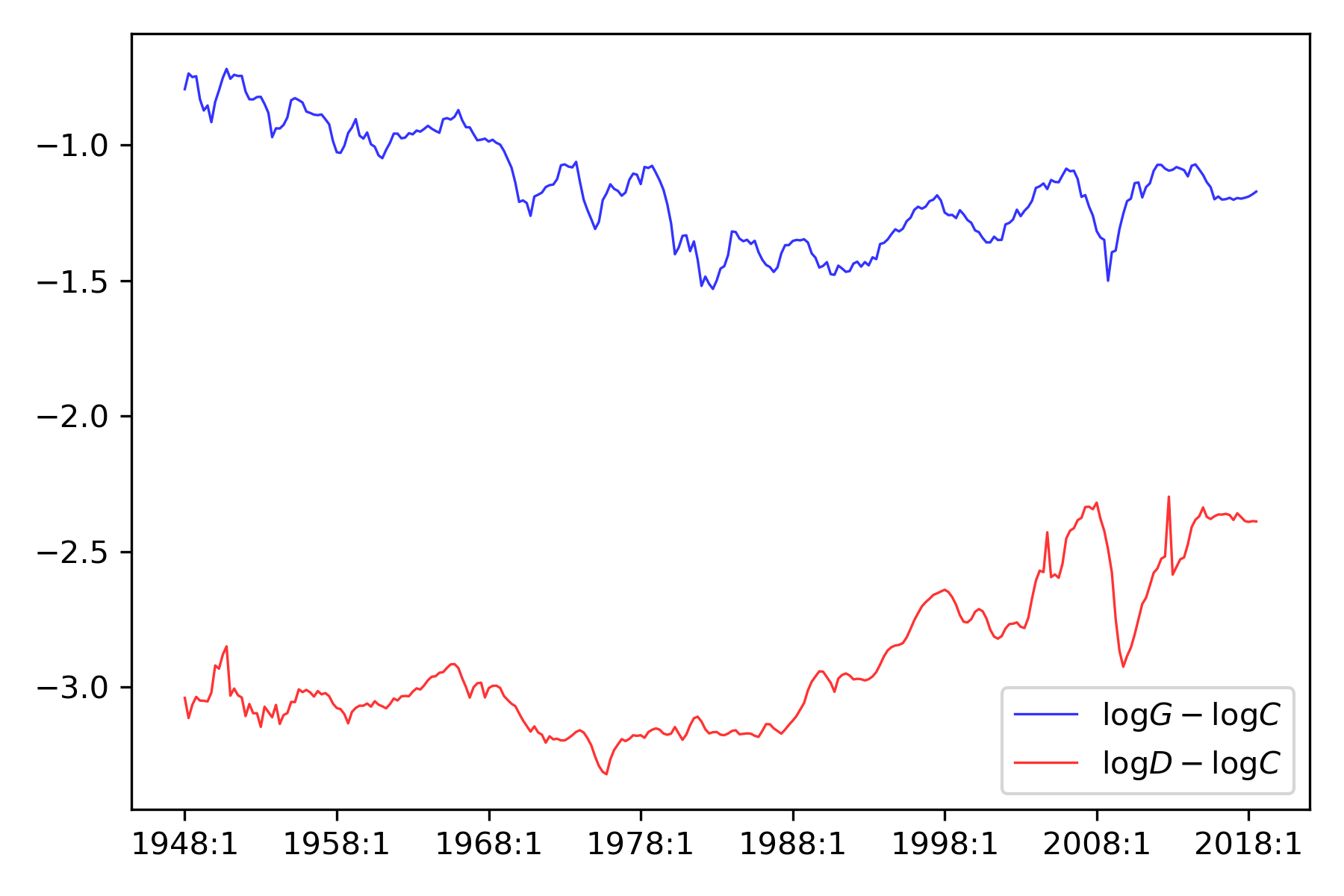
Fig. 6.1 Time series for the i) logarithm of proprietor’s income plus corporate profits relative to consumption (blue) and ii) the logarithm of personal dividend income relative to consumption (red).

We deployed the following steps.

i) Let

\[\begin{split}Z_{t+1} = \begin{bmatrix} \log C_{t+1} - \log C_t \\ \log G_{t+1} - \log C_{t+1} \\ \log D_{t+1} - \log C_{t+1} \end{bmatrix}\end{split}\]

where \(C_t\) is consumption, \(G_t\) is business income, and \(D_t\) is personal dividend income. Business income is measured as proprietor’s income plus corporate profits per capita. Dividends are personal dividend income per capita. The time series are quarterly data from 1948 Q1 to 2018 Q3.[12][13]

ii) Let

\[\begin{split}X_t = \begin{bmatrix} Z_t \\ Z_{t-1} \\ Z_{t-2} \\ Z_{t-3} \\ \log G_{t-4} - \log C_{t-4} \\ \log D_{t-4} - \log C_{t-4} \end{bmatrix}.\end{split}\]

Express a vector autoregression as

\[\begin{split}X_{t+1} & = {\mathbb H} + {\mathbb A} X_t + {\mathbb B} W_{t+1} \\ Z_{t+1} & = {\mathbb D}X_t + {\mathbb F} W_{t+1}\end{split}\]

where \({\mathbb A}\) is a stable matrix (i.e., its eigenvalues are all bounded in modulus below unity) and \({\mathbb B}{\mathbb B}'\) is the innovation covariance matrix. Let selector matrix \({\mathbb J}\) verify \(Z_{t+1} = {\mathbb J} X_{t+1}\). The implied mean \(\mu\) of the stationary distribution for \(X\) is

\[\mu = (I - {\mathbb A})^{-1} {\mathbb H}.\]

The covariance matrix \(\Sigma\) of the stationary distribution of \(X\) solves a discrete Lyapunov equation

\[\Sigma = {\mathbb A} \Sigma {\mathbb A}' + {\mathbb B}{\mathbb B}'.\]

iii) \(\log C_t, \log G_t, \log D_t\) are cointegrated. Each of \(\log C_t, \log G_t, \log D_t\) is an additive functional in the sense of chapter Processes with Markovian increments. Each has an additive decomposition into trend, martingale, and stationary components that can be constructed using a method described in chapter Processes with Markovian increments. Trend and martingale components of the three series are identical by construction. The innovation to the martingale process is identified as the only shock having long-term consequences.

The conjugate prior approach described above does not generate a posterior for which either the prior or the implied posteriors for the matrix \({\mathbb A}\) has stable eigenvalues with probability one. We therefore modify that approach to impose that \({\mathbb A}\) is a stable matrix. We do this by rescaling the posterior probability so that it integrates to one over the region of the parameter space for which \({\mathbb A}\) is stable. We in effect condition on \({\mathbb A}\) being stable. This is easy to implement by rejection sampling.[14]

The standard deviation of the martingale increment is a nonlinear function of parameters in \(({\mathbb A}, {\mathbb B})\). We construct a posterior distribution via Monte Carlo simulation. We draw from the posterior of the multivariate regression system and, after conditioning on stability of the \({\mathbb A}\) matrix, compute the nonlinear functions of interest. From the simulation, we construct joint histograms to approximate posterior distributions of functions of interest.[15]

In Fig. 6.2, we show posterior histograms for the standard deviations of shocks to short-term consumption growth and of the martingale increment to consumption. The standard deviation of the short-term shock contribution is about one-half that of the standard deviation of the martingale increment. Fig. 6.2 tells us that short-term risk can be inferred with much more accuracy than is long-term risk. This evidence says that while there could be a long-run risk component to consumption, it is poorly measured. The fat tail in right of the distribution of the long-run standard deviation is induced by Monte Carlo draws for which some eigenvalues of \(\mathbb A\) have absolute values very close to unity. [16]

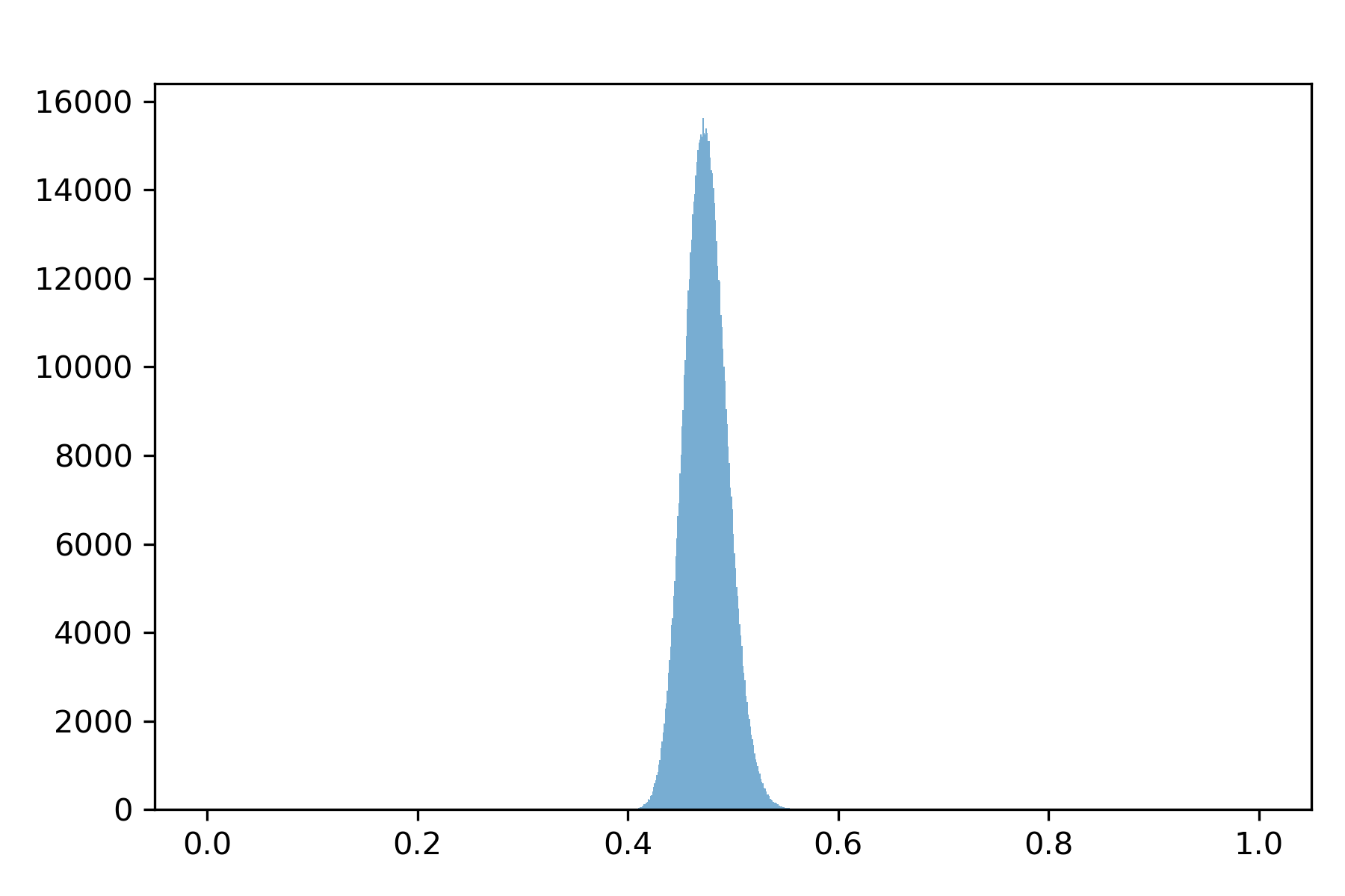
Fig. 6.2 Posterior density for conditional standard deviation of consumption growth.

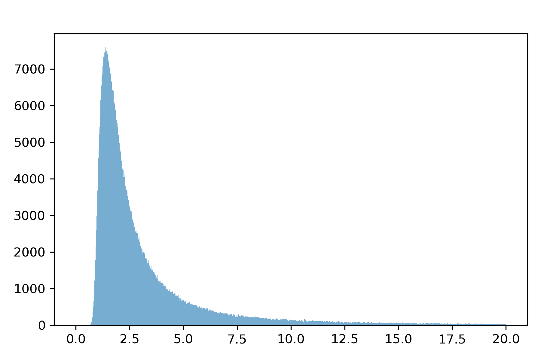
Fig. 6.3 Posterior distribution for the standard deviation of the martingale increment.

Remark 6.3

Carter and Kohn [1994] proposed an extension of the preceding method that is applicable to situations in which a state vector \(X_t\) is hidden. A Carter and Kohn [1994] approach would iterate on the following steps:

• Conditioned on parameters and a fixed data sample, use inputs into the Kalman smoother to simulate hidden states.[17]

  • First draw randomly \(X_T\) given \(\{Z_t : t=1,2,... T \}\) from the solution to the Kalman filtering problem.

  • Working backwards, for \(t=T-1, T-2,... 1\), draw \(X_t\) given \(X_{t+1}\) and \(Z_{t+1}\) conditioned on \(\{Z_\tau : \tau =1,2,... t \}\) using the conditional expectation implied by (6.12) and covariance matrix (6.13).

• Conditioned on data and hidden states, use the conjugate prior approach described above to simulate unknown parameters.

Successive iterations on this algorithm form a Markov process with a state vector consisting of the hidden states and the parameters. Under appropriate regularity conditions, the Markov process has a stationary distribution to which the Markov process formed by the preceding iterations converges. That stationary distribution is the joint posterior distribution of hidden states and parameter values. We are interested in the marginal posterior distributions over parameter values.[18]

6.5. VAR Regimes

Following and , suppose that there are multiple VAR regimes \(({\mathbb A}_i, {\mathbb B}_i, {\mathbb D}_i, {\mathbb F}_i)\) for \(i=1,2,...,n\), where indices \(i\) are governed by a Markov process with transition matrix \(\mathbb{P}\). In regime \(i\) we have

\[\begin{split}X_{t+1} = {\mathbb A}_i X_t + {\mathbb B}_i W_{t+1} \\ Y_{t+1} - Y_t = {\mathbb D}_i X_{t} + {\mathbb F}_i W_{t+1},\end{split}\]

where \(\{W_{t+1}\}_{t=0}^\infty\) is an i.i.d. sequence of \(\mathcal{N}(0,I)\) random vectors conditioned on \(X_0\), and \(F_i\) is nonsingular.

We can think of \(X_t\) and a regime indicator \(Z_t\) jointly as forming a Markov process. When regime \(i\) is realized, \(Z_t\) equals a coordinate vector with one in the \(i^{th}\) coordinate and zeros at other coordinates. We study a situation in which regime indicator \(Z_t\) is not observed. Let \(Q_t\) denote an \(n\)-dimensional vector of probabilities over the hidden states \(Z_t\) conditioned on \(Y^t\), \(X_0\), and \(Q_0\), where \(Q_0\) is the date zero vector of initial probabilities for \(Z_0\). Equivalently, \(Q_t\) is \(E(Z_t \vert Y^t, X_0, Q_0)\).

The vector of conditional probabilities \(Q_t\) solves a filtering problem. We describe the solution of this problem by representing \((X_t,Q_t)\) as a Markov process via the following four steps.

1. Find the joint distribution for \((Z_{t+1},Y_{t+1} - Y_{t)\) conditioned on \((Z_t,X_t)\). Conditional distributions of \(Z_{t+1}\) and \(Y_{t+1} \) are statistically independent by assumption. Conditioned on \(Z_t\), \(X_t\) conveys no information about \(Z_{t+1}\) and thus the conditional density of \(Z_{t+1}\) is given by entries of \(\mathbb{P}'Z_t\). Conditioned on \(Z_t = i\), \(Y_{t+1} \) is normal with mean \(D_i X_t\) and covariance matrix \(F_i(F_i)'\). Let \(\psi_i(y^*,X_t)\) be the normal density function for \(Y_{t+1}-Y_t\) conditioned on \(X_t\) when \(Z_t\) is in regime \(i\). We can write the joint density conditioned on \((Z_t, X_t)\) as:

\[\begin{split}\begin{matrix} \underbrace{(\mathbb{P}'Z_t)} & \times & \underbrace{(Z_t)' \text{vec} \left\{ \psi_i(y^*,X_t) \right\}} \\ \uparrow & & \uparrow \\ Z_{t+1} \ \ \text{density} & & Y_{t+1} -Y_t \ \ \text{density} \end{matrix}\end{split}\]

where \(\text{vec}(r_i)\) is a column vector with \(r_i\) in the \(i^{th}\) entry. We have imposed conditional independence by forming a joint conditional distribution as a product of two conditional densities, one for \(Z_{t+1}\) and one for \(Y_{t+1}-Y_t\).

2. Find the joint distribution of \(Z_{t+1}, Y_{t+1}-Y_t\) conditioned on \((X_t,Q_t)\). Since \(Z_t\) is not observed, we form the appropriate average of the above conditioned on the \(Y^t, X_0, Q_0\):

\[\mathbb{P}' \text{diag}\{Q_t\} \text{vec} \left\{ \psi_i(y^*,X_t) \right\}\]

where \(\text{diag}\{Q_t\}\) is a diagonal matrix with components of \(Q_t\) on the diagonal. Thus, \(Q_t\) encodes all pertinent information about the time \(t\) regime \(Z_t\) that is contained in \(Y^t\), \(X_0\) and \(Q_0\). Notice that conditional on \((X_t,Q_t)\), random vectors \(Y_{t+1}-Y_t\) and \(Z_{t+1}\) are not statistically independent.

3. Find the distribution of \(Y_{t+1}-Y_t\) conditioned on \((X_t,Q_t)\). Summing the above over hidden states gives

\[(\mathbf{1}_n)'\mathbb{P}' \text{diag}\{Q_t\} \text{vec} \left\{ \psi_i(y^*,X_t) \right\} = Q_t\cdot \text{vec} \left\{ \psi_i(y^*,X_t) \right\}.\]

Thus, the distribution for \(Y_{t+1}-Y_t\) conditioned on \((X_t, Q_t)\) is a mixture of normals in which, with probability given by the \(i^{th}\) entry of \(Q_t\), \(Y_{t+1}-Y_t\), is normal with mean \(D_i X_t\) and covariance matrix \(F_i{F_i}'\). Similarly, the conditional distribution of \(X_{t+1}\) is a mixture of normals.

4. Obtain \(Q_{t+1}\) by dividing the joint density for \((Y_{t+1}-Y_t,Z_{t+1})\) conditioned on \((X_t,Q_t)\) by the marginal density for \(Y_{t+1}-Y_t\) conditioned on \((X_t, Q_t)\). Division gives the density for \(Z_{t+1}\) conditioned \((Y_{t+1}-Y_t, X_t,Q_t)\), which in this case is just a vector \(Q_{t+1}\) of conditional probabilities. Thus, we are led to the recursion

(6.22)\[Q_{t+1} = \left( \frac{1}{Q_t\cdot \text{vec} \left\{ \psi_i(Y_{t+1}, X_t) \right\}}\right) \mathbb{P}' \text{diag}(Q_t) \text{vec} \left\{ \psi_i(Y_{t+1}, X_t) \right\}.\]

Taken together, steps (3) and (4) provide the one-step-transition equation for Markov state \((X_{t+1}, Q_{t+1})\). As indicated in step (3), \(Y_{t+1} \) is a mixture of normally distributed random variables. As argued in step (4) the vector \(Q_{t+1}\) is an exact function of \(Y_{t+1} \), \(Q_t\), and \(X_t\) that is given by the above formula (6.22).

---

[1]

Many expositions of Kalman filtering assume that \(BF' = 0\). We shall study some interesting examples in which \(BF' \neq 0\).

[2]

The process \(\{ X_t, t=0,1, 2, \ldots \}\) is also Markov.

[3]

This amounts to dividing the joint distribution for \((X_{t+1}, Z_{t+1} )\) conditioned on \(Q_t\) by the marginal density for \(Z_{t+1}\) conditional on \(Q_t\).

[4]

Presentations of multivariate regression theory often report the transpose of this matrix. Those presentations pre-multiply coefficients by regressors whereas as Kalman filtering representations post-multiply by regressors.

[5]

Let \(z\) be an \(N \times 1\) random vector with multivariate normal probability density \( f(z ; \mu, \Sigma) = (2 \pi)^{-(\frac{N}{2})} \det ( \Sigma)^{-(\frac{1}{2})} \exp \left( -.5 (z -\mu)' \Sigma^{-1} (z- \mu) \right) \) where \(\mu = E z \equiv \int z f(z ; \mu, \Sigma) \, d z \) is the mean of \(z\) and \(\Sigma = E (z - \mu) (z-\mu)' \equiv \int (z - \mu) (z-\mu)' f(z ; \mu, \Sigma) \, d z \) is the covariance matrix of \(z\). For integer \(j \in [2, \ldots, N-1]\), partition \(z\) as \(z = \begin{bmatrix}z_1 \cr z_2\end{bmatrix}\), where \(z_1\) is an \((N-j) \times 1 \) vector and \(z_2\) is a \(j \times 1 \) vector. Let \( \mu = \begin{bmatrix}\mu_1 \cr \mu_2 \end{bmatrix} , \Sigma = \begin{bmatrix} \Sigma_{11} & \Sigma_{12} \cr \Sigma_{21} & \Sigma_{22} \end{bmatrix} \) be corresponding partitions of \(\mu\) and \(\Sigma\). The marginal densities of the random vectors \(z_1\) and \(z_2\) are \(f(z_1 ; \mu_1, \Sigma_{11})\) and \(f(z_2 ; \mu_2, \Sigma_{22})\), respectively, where \(f( z_i ; \mu_i, \Sigma_{ii})\) denotes a multivariate normal density with mean vector \(\mu_i\) and covariance matrix \(\Sigma_{ii}\). The conditional density of \(z_1\) given \(z_2\), denoted \(f(z_1 | z_2; \hat \mu_1, \hat \Sigma_{11})\), is multivariate normal with mean \( \hat \mu_1 = \mu_1 + \beta ( z_2 - \mu_2) \) and covariance matrix \( \hat \Sigma_{11} = \Sigma_{11} - \Sigma_{12} \Sigma_{22}^{-1} \Sigma_{21} = \Sigma_{11} - \beta \Sigma_{22} \beta' \) where \(\beta = \Sigma_{12} \Sigma_{22}^{-1} \) is an \((N- j) \times j\) matrix of population regression coefficients of \(z_1 -\mu_1\) on \(z_2- \mu_2\). Here \(\hat \mu_1 = E z_1 | z_2\) and \(\hat \Sigma_{11} = E [ (z_1 - \hat \mu_1) (z_1 - \hat \mu_1)' ]| z_2 \).

[6]

The logarithm of time \(j\) component of \(L_t\) is evidently \( \log \psi(Z_{j} \mid H + D {\overline X}_{j-1}) = - .5 m \log (2 \pi) - .5 \log \det (\Omega_{j-1}) \) \( - .5 (Z_j - H - D \overline X_{j-1})' \Omega_{j-1}^{-1} (Z_j - H - D \overline X_{j-1}) \)

[7]

This stochastic process is not ergodic, being a mixture of statistical models like those described by Proposition 1.3. In the present setting, conditioning on invariant events means knowing parameters, an assumption incompatible with posing a statistical learning problem.

[8]

This factorization can be implemented as a Cholesky decomposition.

[9]

A decision-maker who does not know the underlying parameters in the matrices \(A, B, D, F, H\) continues to have a Markov decision problem except that \(b_t,c_t,d_t\) must now be included along with the state vector \(X_t\).

[10]

Such a procedure can result in estimators that are inadmissible.

[11]

Box and Tiao [1992] discuss improper priors that include the specification for the regression model here.

[12]

Our consumption measure is nondurables plus services consumption per capita. The nominal consumption data come from BEA’s NIPA Table 1.1.5 and their deflators from BEA’s NIPA Table 1.1.4. The business income data with IVA and CCadj are from BEA’s NIPA Table 1.12. Personal dividend income data were obtained from FRED’s B703RC1Q027SBEA. Population data comes from FRED’s CNP16OV.

[13]

By including proprietors’ income in addition to corporate profits, we used a broader measure of business income than Hansen et al. [2008] who used only corporate profits. Hansen et al. [2008] did not include personal dividends in their VAR analysis.

[14]

Another approach that we don’t use here would be to modify how we construct the likelihood function. Currently, the likelihood function conditions on the initial \(X_0\). We could instead impose that \(X_0\) is described by the stationary distribution associated with a stable \(A\) matrix.

[15]

We could also have used change in variables formulas to deduce posterior distributions of interest, but that would have involved substantial pencil and paper work and require additional numerical computation.

[16]

Bounding absolute values of these eigenvalues to be less than a pre-specified number strictly less than one would thin the right tail. Doing that amounts indirectly to imposing a particular prior on the size of long-run risk.

[17]

A Kalman smoother works backward to construct a probability distribution for hidden states \(X_t\) for \(t=0,1,..., T-1\) conditioned on a complete sample of observations \(\{Z_t : t=1,2,... T \}\).

[18]

A Carter and Kohn [1994] simulation approach is an example of a Gibbs sampler.