Manuscript

Authors: Lars Peter Hansen and Thomas J. Sargent

Date: July 2024 \(\newcommand{\eqdef}{\stackrel{\text{def}}{=}}\)

For nonlinear stochastic models, impulse responses are themselves stochastic. The manuscript provides characterizations of these responses in both discrete and continuous time. These characterizations are central inputs into marginal valuations, whereby endogenous state variables are represented as asset prices with stochastic payoffs and discounting. These resulting formulas provide representations for policy relevant variables such as the social cost of climate change and the social value of research and development. The derivations show how robustness concerns impact the valuations.

---

1 Introduction

Partial derivatives of value functions measure marginal valuations and appear in first-order conditions of Markov decision problems. They feature prominently in max-min formulations of robust control problems. They can be used to measure losses from suboptimal choices. For example, the social cost of global warming is the important contributor to calculations of the social cost of carbon emissions often inferred from marginal impacts of fossil fuel emissions on climate indicators measured as potentially uncertain damages to economic opportunities in the future. By importing insights about stochastic nonlinear impulse response functions and from asset pricing methods for valuing uncertain cash flows, this chapter constructs representations of partial derivatives and decompositions of them by i) time horizon and ii) marginal contributions to future utilities.

2 Discrete time

We first consider a discrete-time specification.

2.1 Discrete Markov dynamics

We start with Markov process

(1)\[\begin{split}X_{t+1} = \psi(X_t, W_{t+1}), \\ Y_{t+1} - Y_t = \kappa(X_t, W_{t+1}),\end{split}\]

where there are \(n\) components of \(X\) and \(Y\) is scalar.

2.2 Discrete variational dynamics

Let \(\Lambda\) denote the first variational process for \(X\), and let \(\Delta\) denote the first variational process for \(Y\). These variational processes are the ingredients to stochastic impulse responses to small changes in the underlying state variables. We compute them by “differentiating” in a generalized sense that accommodates the underling stochastic structure.
To obtain a recursive representation for \((\Lambda, \Delta),\) we by differentiate (1) and apply the chain rule:

(2)\[\begin{split}\Lambda_{t+1} = \frac {\partial \psi}{\partial x'} (X_t, W_{t+1}) \Lambda_t \\ \Delta_{t+1} - \Delta_t = \frac {\partial \kappa}{\partial x}(X_t, W_{t+1}) \cdot \Lambda_t \end{split}\]

In this calculation, \(\Lambda_{t+1}\) and \(\Delta_{t+1}\) are stochastic as they inherit the stochastic dependence of \(X_{t+1}\) and \(Y_{t+1}.\) By differentiating the process at a given calendar date, we are allowing for date \(t\) variables to change as a function of date \(t\) information.

To obtain alternative stochastic (local) impulse response functions, we initialize \(({\Lambda_0}', \Delta_0)'\) to be one of the coordinate vectors that depends on one of the initial states that we want to perturb. Then \(({\Lambda_t}', \Delta_t)'\) is the date \(t\) state vector stochastic response to the perturbation of the initial value of the component.

To perturb \(Y_0,\) we can set \(\Lambda_0 = 0\) and \(\Delta_0=1;\) then \(\Lambda_t = 0\) and \(\Delta_t = 1\) for all \(t\). Alternatively, if we initialize \(\Lambda_0\) be a coordinate vector and \(\Delta_0 =0,\) then the response \(\Delta_t\) will be a stochastic process.

Remark 1

The evolution of the variational processes is nonstochastic if \( \frac {\partial \psi}{\partial x'}\) and \( \frac {\partial \kappa}{\partial x}\) are constant as is true when \(\psi\) and \(\kappa\) are affine in \(x\). Otherwise, variational processes are stochastic.

2.3 Marginal valuation

We use stochastic impulse responses to provide an “asset pricing” representation of partial derivatives of a value function with respect to one of the components of \(X_0\). Consider a value function that satisfies:

(3)\[\begin{split}\begin{align} V(X_t) + Y_t = & \exp(-\delta) \mathbb{E} \left[ V(X_{t+1}) + Y_{t+1} \mid X_t \right] \\ & + [1 - \exp(-\delta)] \left[ U(X_t) + Y_t \right]. \end{align}\end{split}\]

This value function need not coincide with a solution to an optimal control problem. It could just be the evaluation of some non-optimal decision rule associated with a stochastic equilibrium. Marginal valuation is still used as part of a local policy analysis.

Differentiate both sides of this (3) with respect to \(X_t\) and \(Y_t\) and form dot products with appropriate variational counterparts:

(4)\[\begin{split}\begin{align} \frac{\partial V}{\partial x}(X_t) \cdot \Lambda_t + \Delta_t = & \exp(-\delta) \mathbb{E}\left[ \frac{\partial V}{\partial x}(X_{t+1}) \cdot \Lambda_{t+1} + \Delta_{t+1} \mid X_t, \Lambda_t, \Delta_t \right] \\ & + [1 - \exp(-\delta)]\left[\frac{\partial U}{\partial x}(X_t) \cdot \Lambda_t + \Delta_t \right] \end{align} \end{split}\]

View equation (4) as a stochastic difference equation and solve it forward for \(\frac{\partial V}{\partial x}(X_t) \cdot \Lambda_t + \Delta_t:\)

(5)\[\begin{split}\begin{align*} & \frac{\partial V}{\partial x}(X_t) \cdot \Lambda_t + \Delta_t \\ & = [1 - \exp(-\delta)]\sum_{\tau = 0}^\infty \mathbb{E}\left( \exp(-\tau \delta) \left[\frac{\partial U}{\partial x}(X_{t+\tau}) \cdot \Lambda_{t+\tau} + \Delta_{t + \tau}\right] \mid X_t, \Lambda_t, \Delta_t \right) \end{align*}\end{split}\]

Initialize \(\Lambda_0 = \mathrm{e}_i\) where \(\mathrm{e}_i\) is a coordinate vector with a one in position \(i\) and \(\Delta_0 = 0.\) We now have represented the partial derivative of the value function as:

\[\frac{\partial V}{\partial x_i}(x) = [1 - \exp(-\delta)]\sum_{t = 0}^\infty \exp(-t \delta) \mathbb{E}\left[ \frac{\partial U}{\partial x}(X_{t}) \cdot \Lambda_{t} + \Delta_t \mid X_0 = x, \Lambda_0 = \mathrm{e}_i, \Delta_0 = 0 \right]\]

This resembles an asset pricing formula in which

\[\begin{split}\left\{\exp(-\delta t)\begin{bmatrix} \Lambda_t \\ \Delta_t \end{bmatrix} : t \ge 0 \right\}\end{split}\]

acts as a vector stochastic discount factor process and the marginal contribution

\[\begin{split}\left\{ [1 - \exp(-\delta)]\begin{bmatrix} \frac{\partial U}{\partial x}(X_{t}) \\ \Delta_t \end{bmatrix} : t \ge 0\right\}\end{split}\]

acts as a vector stochastic cash flow process. The stochastic impulse response tells the marginal state vector response at date \(t\) to changing the \(i^{th}\) state vector component at date zero, while the vector of marginal cash flows at date \(t\) measures the impact on utility of a marginal change in the date \(t\) state vector.

Remark 2

Sometimes it is convenient to apply summation by parts:

\[\begin{split}\begin{align*} & [1 - \exp(-\delta)]\sum_{\tau = 0}^\infty \mathbb{E}\left( \exp(-\tau \delta) \Delta_{t + \tau} \mid X_t, \Lambda_t, \Delta_t \right) \\ & = \sum_{\tau = 1}^\infty \mathbb{E}\left[ \exp(-\tau \delta) \left(\Delta_{t + \tau} - \Delta_{t+\tau -1} \right) \mid X_t, \Lambda_t, \Delta_t \right] + \Delta_t \\ & = \sum_{\tau = 1}^\infty \mathbb{E}\left[ \exp(-\tau \delta) \frac{\partial \kappa}{\partial x}(X_{t+\tau-1}, W_{t+\tau})\cdot \Lambda_{t+ \tau} \mid X_t, \Lambda_t, \right] + \Delta_t . \end{align*}\end{split}\]

Substituting into (5) gives:

\[\begin{split}\frac{\partial V}{\partial x}(X_t) \cdot \Lambda_t + \Delta_t = [1 - \exp(-\delta)]\sum_{\tau = 0}^\infty \mathbb{E}\left[ \exp(-\tau \delta) \frac{\partial U}{\partial x}(X_{t+\tau}) \cdot \Lambda_{t+\tau} \mid X_t, \Lambda_t, \right] \\ + \sum_{\tau = 1}^\infty \mathbb{E}\left[ \exp(-\tau \delta) \frac{\partial \kappa}{\partial x}(X_{t+\tau-1}, W_{t+\tau})\cdot \Lambda_{t+ \tau} \mid X_t, \Lambda_t, \right] + \Delta_t.\end{split}\]

3 Continuous time

A continuous-time counterpart allows us to draw a distinction between small shocks (Brownian increments) and large shocks (Poisson jumps). Formally, we consider a continuous-time specification with Brown motion shocks, in other words, diffusion dynamics. We then allow for jumps by treating them as terminal conditions where we impose continuation values conditioned on a jump taking place. The possibility of a jump will contribute to the value function computation. After developing the basic approach we extend the analysis to include robustness in the valuation.

3.1 Diffusion dynamics

As a part of a more general derivation, we begin with state dynamics modeled as a Markov diffusion:

\[\begin{split}\begin{align*} dX_t & = \mu(X_t) dt + \sigma(X_t) dW_t \\ dY_t & = \nu(X_t) dt + \varsigma(X_t) \cdot dW_t. \end{align*}\end{split}\]

As for discrete time, these dynamics might or might not be outcomes of an optimization problem.

3.2 Variational process

Following [Borovička et al., 2014], we construct marginal impulse response functions using what are called variational processes. We build the dynamics for what is called the first valuation process, \(\Lambda\) by following the construction in [Fournie et al., 1999]. The first valuation process tells the marginal impact on future \(X\) of a marginal change in one of the initial states analogous to the \(\Lambda\) process that we constructed in discrete time. Thus this process has the same number of components as \(X\). By initializing the process at one of the alternative coordinate vectors, we again isolate an initial state of interest.[1]

The drift for the \(i^{th}\) component of \(\Lambda\) is

\[\lambda' {\frac {\partial \mu_i} {\partial x} }(x) \]

and the coefficient on the Brownian increment is

\[\lambda' \frac {\partial \sigma_i }{\partial x}(x)\]

for \(\lambda\) a hypothetical realization of \(\Lambda_t\) and \(x\) a hypothetical realization of \(X_t,\) where \('\) denotes vector or matrix transposition. The implied evolution of the process \(\Lambda^i\) is\footnote{Since we are working with an instantaneous evolution with Brownian increments, we are implicitly appealing to a formalism known as Malliavin calculus.}

\[d\Lambda_{t}^i = \left(\Lambda_t\right)'\frac{\partial \mu_i}{\partial x}(X_t) dt + \left({\Lambda_t}\right)'\frac{\partial \sigma_i}{\partial x}(X_t) dW_t.\]

With the appropriate stacking, the drift for the composite process \((X,\Lambda)\) is:

(6)\[\begin{split}\mu^a(x,\lambda) \overset{\text{def}}{=} \begin{bmatrix} \mu(x) \\ \lambda'{\frac {\partial \mu_i} {\partial x} }(x) \\ ... \\ \lambda'{\frac {\partial \mu_n} {\partial x} }(x) \end{bmatrix},\end{split}\]

and the composite matrix coefficient on \(dW_t\) is given by

(7)\[\begin{split}\sigma^a(x,\lambda) \overset{\text{def}}{=} \begin{bmatrix} \sigma(x) \\ \lambda'\frac {\partial \sigma_1 }{\partial x}(x)\\ ... \\ \lambda' \frac {\partial \sigma_n }{\partial x}(x) \end{bmatrix}.\end{split}\]

Let \(\Delta\) be the scalar variational process associated with \(Y.\) Then

\[d \Delta_t = \Lambda_t \cdot \frac {\partial \nu}{\partial x} (X_t)dt + {\Lambda_t}' \frac {\partial \varsigma}{\partial x'} dW_t \]

3.3 An initial representation of a partial derivative

Consider the evaluation of discounted utility where the instantaneous contribution is \(U(x)\) where \(x\) is the realization of a state vector \(X_t\). The function \(U\) satisfies a Feynman-Kac (FK) equation:

(8)\[\begin{align} 0 = & \delta \left[U(x) + y\right] - \delta \left[V(x) + y \right] \mu(x) \cdot \frac {\partial V}{\partial x}(x) + \nu(x) \cr &+ {\frac 1 2 }{\rm trace}\left[\sigma(x)' \frac {\partial^2 V}{\partial x \partial x'}(x) \sigma(x) \right]. \end{align}\]

As in the discrete-time example, we want to represent

\[V_{x_i}(x) = {\frac {\partial V}{\partial x_i}}(x) \]

as an expected discounted value of a marginal impulse responses of future \(X_t\) to a marginal change of the \(i^{th}\) coordinate of \(x.\)

By differentiating Feynman-Kac equation (8) with respect to each coordinate, we obtain a vector of equations one for each state variable. We then form the dot product of this vector system with respect to \(m\) to obtain a scalar equation system that is of particular interest. The resulting equation is a Feynman-Kac equation for the scalar function:

\[\lambda \cdot \frac {\partial V}{\partial x}\]

as established in the Appendix. Given that the equation to be solved involves both \(\lambda\) and \(x\), this equation uses the diffusion dynamics for the joint process \((X,\Lambda)\).

The solution to this Feynman-Kac equation takes the form of a discounted expected value:

(9)\[\frac {\partial V}{\partial x}(X_0) \cdot \Lambda_0 + \Delta_0 = \delta \int_0^\infty \exp( - \delta t ) {\mathbb E} \left[ \frac {\partial U}{\partial x} (X_{t}) \cdot \Lambda_{t} + \Delta_t \mid X_0, \Lambda_0, \Delta_0 \right] dt. \]

By initializing the state vector \(\Lambda_0\) to be a coordinate vector of zeros in all entries but entry \(i\) and \(\Lambda_0 = 0\), we obtain the formula we want, which gives the partial derivative as a discounted present value using \(\delta\) as the discount rate. The contribution, \(\Lambda_{t},\) is the marginal response of the date \(t\) state vector to marginal change in the \(i^{th}\) component of the state vector at date zero. The marginal change in the date \(t\) state vector induces marginal reward at date \(t\):

\[\delta \frac {\partial U}{\partial x} (X_{t})\cdot \Lambda_{t} + \Delta_t\]

which provides us with a useful interpretation as an asset price. The process \(\Lambda\) gives a vector counterpart to a stochastic discount factor process and \(\delta \frac {\partial U}{\partial x} (X_{t}) + \Delta_t\) gives the counterpart to a cash flow to be valued.

One application of representation (9) computes the discounted impulse response:

\[\delta \exp( - \delta t ) {\mathbb E} \left[ \frac {\partial U}{\partial x_j} (X_{t}) \cdot \Lambda_{t} \mid X_0, \Lambda_0, \Delta_0 \right]. \]

for \(t \ge 0\) and for \(j=1,2,...,n\) along with

\[\delta \exp( - \delta t ) {\mathbb E} \left[ \Delta_t \mid X_0, \Lambda_0, \Delta_0 \right] \]

for \(t \ge 0\) as an intertemporal, additive decomposition of the marginal valuation of one of the state variables as determined by an initialization of \(\Lambda_0.\)

Remark 3

Representations similar to (7) appear in the sensitivity analyses of options prices. See [Fournie et al., 1999].

3.4 Robustness

We next consider a general class of drift distortions that can help us study model misspecification concerns. We initially explore the consequences of exogenously-specified drift distortion. After that, we show how such a distortion can emerge endogenously as a decision maker’s response to concerns about model misspecifications.

We introduce an exogenously specified drift distortion process \(H\) into the diffusion dynamics:

\[\begin{split}\begin{align*} &d X_t = \mu(X_t)dt + \sigma(X_t) H \left( \bar{X}_t \right) dt + \sigma(X_t) dW_t \\ &d \overline{X}_t = \bar{\mu}\left( \overline{X}_t \right) dt + \bar{\sigma}\left(\overline{X}_t \right) dW_t. \end{align*}\end{split}\]

By imitating our earlier analysis, we can associate with this joint system \((X, \overline{X})\) a composite variational process \((\Lambda, \overline{\Lambda}).\) To study endogenous state variable sensitivity, we are especially interested in the \(M\) component, not the \(\overline{\Lambda}_t\) process. Notice that if we set \(\overline{\Lambda}_0 = 0\), then \(\overline{\Lambda}_t = 0\) for \(t > 0.\)

The evolution for the variational process component \(\Lambda\) becomes:

\[d\Lambda_{t}^i = \left(\Lambda_t\right)'\left[\frac{\partial \mu_i}{\partial x}(X_t) + \frac{\partial \sigma_i}{\partial x}(X_t) H\left( \overline{X}_t \right) \right]dt + \left(\Lambda_t\right)'\frac{\partial \sigma_i}{\partial x}(X_t) dW_t.\]

Importantly, there is no contribution from differentiating \(H\) with respect to \(x\) since \(H\) only depends on the \(\bar{X}_t\) process.

Remark 4

While we focus on Markov forms of misspecification, this can be relaxed. The misspecification that will most concern a decision maker will have a Markov representation. That helps explain why we make a Markov assumption here.

3.5 Value function derivatives under robustness

We now let the flow term be:

\[\delta \left[ U(x) + y \right] +{\frac \xi 2} \vert H\left( \bar{x} \right) \vert^2.\]

This implies a value function \({\overline V}(x,{\bar x}) + y.\)

Consider another value function that is sometimes used to compute a robustness adjustment to valuation. It coincides with ones sometimes used in robust control problems. This value function solves the HJB equation:

(10)\[\begin{align} 0 = \min_h & \hspace{.2cm} \delta \left[U(x) + y\right] - \delta \left[ V(x) + y \right]+ {\frac \xi 2}|h|^2 + \left[\mu(x) +\sigma(x)h \right] V_x(x) \cr & + \nu(x) + \varsigma(x) \cdot h + {\frac 1 2} {\rm trace} \left[ \sigma (x)' V_{xx}(x) \sigma(x) \right]. \end{align}\]

The first-order conditions for \(h\) in equation (10) imply that

\[\sigma(x)'V_x(x) + \varsigma(x) + \xi h = 0 \]

The solution, \(V,\) of the HJB equation satisfies the Feynman-Kac equation that emerges after we substitute the minimizing \(h\) into the HJB equation:

(11)\[\begin{split}\begin{align} 0 =& \hspace{.2cm} \delta U(x) - \delta V(x) + {\frac \xi 2}|h^*(x) |^2 + \left[\mu(x) +\sigma(x)h^*(x) \right] \cdot V_x(x) \\ & + \left[\nu(x) + \varsigma(x)\cdot h^*(x) \right] + {\frac 1 2} {\rm trace} \left[ \sigma (x)' V_{xx}(x) \sigma(x) \right] , \end{align}\end{split}\]

where

(12)\[h^*(x) = - \frac 1 \xi \left[ \sigma'(x) V_x(x) + \varsigma(x) \right].\]

Consider an exogenously specified drift distortion as in the previous subsection where \(H = h^*\) and stochastic dynamics \(\bar X\) satisfy a consistency requirement:

\[\begin{split}\begin{align} {\bar \mu }(x) &= \mu(x) + H(x) \\ {\bar \sigma}(x) &= \sigma(x) \end{align}\end{split}\]

and \({\bar X}_0 = X_0.\)

We now show that when \( H(\bar x) = h^*( \bar x ),\) it is also true that

(13)\[\begin{split}\begin{align} V(x) & = {\overline V}(x,x) \\ V_x(x) & = {\overline V}_x(x,x) \end{align}\end{split}\]

Differentiate equation (11) with respect to \(x\):

\[\begin{split}\begin{align} 0 = & - \delta V_x + \delta U_x + V_{xx}\left(\mu +\sigma h^* \right) + (\mu_x)'V_x + {\rm{mat}} \left\{ \left(\frac {\partial \sigma_i} {\partial x} \right) h^* \right\}'V_x + \frac{\partial \nu}{\partial x} + \frac {\partial \varsigma'} {\partial x} h^* \\ & + {\frac \partial {\partial x}} \left[{\frac 1 2} {\rm trace} \left( \sigma' V_{xx} \sigma \right) \right] \end{align}\end{split}\]

where \(\rm{mat}\) denotes a matrix formed by stacking the column arguments. (This expression uses the first-order conditions for h and an “Envelope Theorem” to cancel some terms.) Take corresponding derivatives of \({\overline V}\) with respect to the first-argument and then substitute \(x={\bar x}\) to obtain (13) when we set \(H(x) = h^*(x).\)

Note that it follows from the second equation in (13) that

\[V_{xx}(x) = {\overline V}_{xx}(x,x) + {\overline V}_{x\bar x}(x,x) \]

Remark 5

We can drop \(\frac{\xi}{2} |H(\overline{X}_t)|^2\) from the flow term that we used to construct \(\overline{V}\) and still obtain the second equality in (13) involving first-derivatives of value functions.

We can now compute representations that we have been seeking by simulating under the endogenously determined worst-case probability specification; we can obtain decompositions of various contributions over time and state vector components based on:

(14)\[\begin{align*} &\frac{\partial \overline{V}}{\partial x}(X_0, \overline{X}_0) \cdot \Lambda_0 + \Delta_0 \cr &= \delta \int_0^\infty \exp(-\delta t) \widetilde{\mathbb{E}} \left[ \frac{\partial U}{\partial x}(X_{t}) \cdot \Lambda_{t} + \Delta_t \mid X_0, \bar{X}_0, \Lambda_0, \Delta_0 \right] dt \end{align*}\]

where set \(\overline{X}_0 = X_0\) and \(\Lambda_0\) equal to one of the coordinate vectors and \(\Delta_0 = 0.\) The mathematical expectation, \(\widetilde{\mathbb{E}}\), is computed under the worst-case stochastic evolution computed by imposing \(H(\overline{X}_t) = h^*(X_t).\)

Remark 6

While we demonstrated that we can treat a drift distortion as exogenous to the original state dynamics, for some applications we will want to view it as a change in the endogenous dynamics that are reflected (12).

Remark 7

By construction, along a simulated path, \(\overline{X}_t = X_t\), which we impose in our numerical calculations. As a consequence, it suffices to simulate \((X,\Lambda)\).

3.6 Allowing IES to differ from unity

Let \(\rho\) be the inverse of the intertemporal elasticity of substitution for a recursive utility specification. The utility recursion is now:

\[\left(\frac{\delta}{1-\rho}\right)\left(\exp\left[(1-\rho)\left[U(X_t)+Y_t\right]\right)\exp\left[(\rho-1)\left[\overline{V}(X_t,\bar{X}_t)+Y_t\right]\right]-1\right) + \overline{\mu}_{v,t} = 0\]

where \(\overline{\mu}_{v,t}\) is the local mean of \(\overline{V}(X,\bar{X}) + Y\) with the robust adjustment discussed above. Compute:

\[\begin{split}\begin{align*} &\frac{\partial}{\partial x}\left(\frac{\delta}{1-\rho}\right)\left(\exp\left[(1-\rho)\left[U(x)+y\right]\right)\exp\left[(\rho-1)\left[\overline{V}(x,\overline{x})+y\right]\right]-1\right) \\ &= \delta\exp\left[(1-\rho)\left[U(x)-\overline{V}(x,\overline{x})\right]\right]\left[\frac{\partial U}{\partial x}(x)-\frac{\partial\overline{V}}{\partial x}(x,\overline{x})\right] \end{align*}\end{split}\]

With this computation, we modify the previous formulas by replacing the subjective discount factor, \(\exp(-t\delta),\) with

\[D_t \eqdef \exp\left(-\int_0^t\delta\exp\left[(1-\rho)\left[U(X_\tau)-\overline{V}(X_\tau,\overline{X}_\tau)d\tau\right]\right]\right).\]

Thus the instantaneous discount rate is now state dependent and depends on the both how the current utility compares to the continuation value and on whether \(\rho\) is greater or less than one. When the current utility exceeds the continuation value, the discount rate is scaled up when \(\rho\) exceeds one and is scaled down when \(\rho\) is less than one. The instantaneous flow term, \(\delta\frac{\partial U}{\partial x}(X_t),\) with

\[ \delta\exp\left[(1-\rho)\left[U(X_\tau)-\overline{V}(X_\tau,\overline{X}_\tau)\right]\right]\frac{\partial U}{\partial x}(X_t).\]

Combining these contributions gives:

\[\begin{align*} & \frac {\partial {\overline V}}{\partial x}\left( X_0, {\overline X}_0 \right) + \Delta_0 \cr & = \delta \int_0^\infty \widetilde{\mathbb E} \left[ D_t \exp\left[(1-\rho)\left[U(X_t)-{\overline V}\left( X_t, {\overline X}_t \right) \right]\right]\frac{\partial U}{\partial x}(X_t) \mid X_0 \Lambda_0, \Delta_0 \right] dt. \end{align*} \]

Remark 8

When we conduct simulations, we can impose that \(\overline{X}_t = X_t\) along with (13), implying that

\[\overline{V}\left(X_\tau,\overline{X}_\tau\right) = V(X_\tau).\]

3.7 Jumps

We study a pre-jump functional equation in which jump serves as a continuation value. We allow multiple types of jumps, each with its own state-dependent intensity. We denote the intensity of a jump of type \(\ell\) by \(\mathcal{J}^\ell(x)\); a corresponding continuation value after a jump of type \(\ell\) has occurred is \(V^\ell(x)+y\). In applications, we’ll compute post-jump continuation value \(V^\ell\), as components of a complete model solution. To simplify the notation, we impose that \(\rho - 1,\) but it is straightforward to incorporate the \(\rho \ne 1\) extension we discussed in the previous subsection.

As in [Anderson et al., 2003], an HJB equation that adds concerns about robustness to misspecifications of jump intensities as well as diffusion dynamics is:

\[\begin{split}\begin{align*} 0 = \min_{h, \, g^\ell \text{ for } \ell=1,...,L} & - \delta V + \delta U + {\frac{\xi}{2}}|h|^2 +\left[\mu +\sigma h\right]\cdot \frac {\partial V}{\partial x} + \nu + \varsigma \cdot h\\ & + {\frac{1}{2}}{\rm trace}\left[\sigma'\frac {\partial^2 V }{\partial x \partial x'}\sigma\right] \\ & + \sum_{\ell=1}^L g^\ell\mathcal{J}^\ell(x)\left[V^\ell - V)\right] \\ & + \xi\sum_{\ell=1}^L\mathcal{J}^\ell(x)\left[1 - g^\ell + g^{\ell}\log g^\ell\right], \end{align*}\end{split}\]

where \(g^\ell \ge 0\) alters the intensity of type \(\ell.\) First-order conditions for the \(g^\ell\)s are

\[\left[V^\ell(x) - V(x)\right] + \xi\log g^{\ell} = 0.\]

First-order conditions for \(h\) remain the same as before.

We again construct a Feynman-Kac equation by substituting in \(h^*(x)\) and \(g^{\ell*}(x)\). Applying an Envelope Theorem to first-order conditions for minimization tells us that neither \(h^*(x)\) nor \(g^{\ell*}(x)\) contribute to the derivatives of the value function. This leads us to:

(15)\[\begin{split}\begin{align*} 0 = & -\delta \frac {\partial V }{\partial x} + \delta \frac {\partial U }{\partial x} + \frac {\partial^2 V }{\partial x \partial x'}\left(\mu +\sigma h^*\right)\\ & + \left( \frac {\partial \mu'}{\partial x} \right) \frac {\partial V }{\partial x} + {\rm{mat}}\left\{\left(\frac{\partial \sigma_i}{\partial x}\right)h^*\right\}' \frac {\partial V }{\partial x}\\ & +\frac{\partial}{\partial x}\left[\frac{1}{2}{\rm trace}\left(\sigma' \frac {\partial^2 V }{\partial x \partial x'} \sigma\right)\right] \\ & +\sum_{\ell=1}^L\frac {\partial \mathcal{J}^{\ell}}{\partial x} g^{\ell*}\left[V^\ell - V\right] \\ & +\sum_{\ell=1}^L\mathcal{J}^{\ell}g^{\ell*}\left[\frac {\partial V^\ell }{\partial x} - \frac {\partial V }{\partial x}\right] \\ & +\xi\sum_{\ell=1}^L\frac {\partial \mathcal{J}^{\ell}}{\partial x} \left[1 - g^{\ell*} + g^{\ell*}\log g^{\ell*}\right]. \end{align*}\end{split}\]

Applying our \((X,\overline{X})\) analysis tells us that the date \(t\) intensity distortion constructed with the minimizing \(g^{\ell*}\) depends on the exogenous state vector \(\overline{X}_t\) rather than on \(X_t\). An Envelope Theorem is again at play here.

It will be enlightening to rewrite equation (15) as:

\[\begin{split}\begin{align*} 0 = & -\left(\delta + \sum_{\ell=1}^L\mathcal{J}^{\ell}g^{\ell*}\right)\frac {\partial V }{\partial x} + \delta \frac {\partial U }{\partial x} \\ & + \frac {\partial^2 V }{\partial x \partial x'}\left(\mu +\sigma h^*\right) + \left( \frac {\partial \mu'}{\partial x}\right)'\frac {\partial V }{\partial x} + {\rm{mat}}\left\{\left(\frac{\partial \sigma_i}{\partial x}\right)h^*\right\}'\frac {\partial V }{\partial x} \\ & + \frac{\partial}{\partial x}\left[\frac{1}{2}{\rm trace}\left(\sigma'\frac {\partial^2 V }{\partial x \partial x'}\sigma\right)\right] \\ & + \sum_{\ell=1}^L\frac {\partial \mathcal{J}^{\ell}}{\partial x} g^{\ell*}\left(V^\ell - V\right) \\ & + \sum_{\ell=1}^L\mathcal{J}^{\ell}g^{\ell*} \frac {\partial V^\ell}{\partial x} \\ & + \xi\sum_{\ell=1}^L \frac {\partial \mathcal{J}^{\ell}}{\partial x}\left[1 - g^{\ell*} + g^{\ell*}\log g^{\ell*}\right]. \end{align*}\end{split}\]

Notice how distorted intensities act like endogenous discount factors in this equation. The last three terms add a flow term to pertinent Feynman-Kac equations via dot products with respect to \(m\). It is significant that these terms do not include derivatives of \(g^{\ell*}\) with respect to \(x\).

For simulating our asset pricing representation of the partial derivatives of the value function, the discounting term becomes state dependent in order to adjust for the jump probabilitites:

\[D_t \eqdef \exp\left( - \int_0^t\left[\delta + \sum_{\ell=1}^L\mathcal{J}^{\ell}(X_u)g^{\ell*}(X_u)\right]du\right),\]

In addition, four flow terms are discounted:

(16)\[\begin{split}\begin{align} & \delta \Lambda_t \cdot U_x(X_t) \\ & + \Lambda_t \cdot \sum_{\ell=1}^L\mathcal{J}^{\ell}_x(X_t)g^{\ell*}(X_t)\left[V^\ell(X_t) - V(X_t)\right] \\ & + \Lambda_t \cdot \sum_{\ell=1}^L\mathcal{J}^{\ell}(X_t)g^{\ell*}(X_t) \frac {\partial V^\ell}{\partial x} (X_t) \\ & + \xi \Lambda_t \cdot\sum_{\ell=1}^L \mathcal{J}^\ell_x (X_t)\left[1 - g^{\ell*}(X_t) + g^{\ell*}(X_t)\log g^{\ell*}(X_t)\right]. \end{align}\end{split}\]

Simulations should be conducted under implied worst-case diffusion dynamics. With multiple jump components, we can decompose contributions to the marginal utility by jump types \(\ell\).

Climate change example

[Barnett et al., 2024] use representations (16) to decompose their model-based measure of the social cost of climate change and the social value of research and development. In their analysis, there are two types of Poisson jumps. One is the discovery of a new technology and the other is recognization of how curved the damage function is for more extreme changes in temperature. A damage function is revealed by a damage jump triggered by a temperature anomaly between 1.5 and 2 degrees celsius. They allow for twenty different damage curves with various curvatures. They display the quantitative importance of each in contributing to the social value of research and development. We report analogous findings for the social cost of climate change measured as the negative of the marginal value of temperature. We take the negative since warming induces damages. While there are twenty one possible jump types, we group them into damage jumps (one through twenty) and a technology jump (twenty one).

Table 1 reports the the contribution of each of the four contributions given on the right side of (16).

\(\xi\)	i	ii(dc)	ii(td)	iii(dc)	iii(td)	iv	sum
\(\infty\)	0.002	0.062	-0.003	0.001	0.003	-0.000	0.064
\(.150\)	0.004	0.143	-0.005	0.000	0.004	-0.029	0.118
\(.075\)	0.007	0.408	-0.004	-0.000	0.004	-0.134	0.280

Table 1: Components to the partial derivative of the value function with respect to the Temperature state variable. The column (dc) includes only the contributions from the damage curve realization jumps, and (td) includes the remaining contribution from the technology discovery jump. All four uncertainty channels are activated.

Fig. 2 The second term in (16) multiplied by -1.

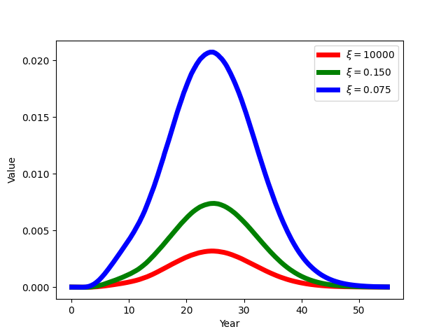
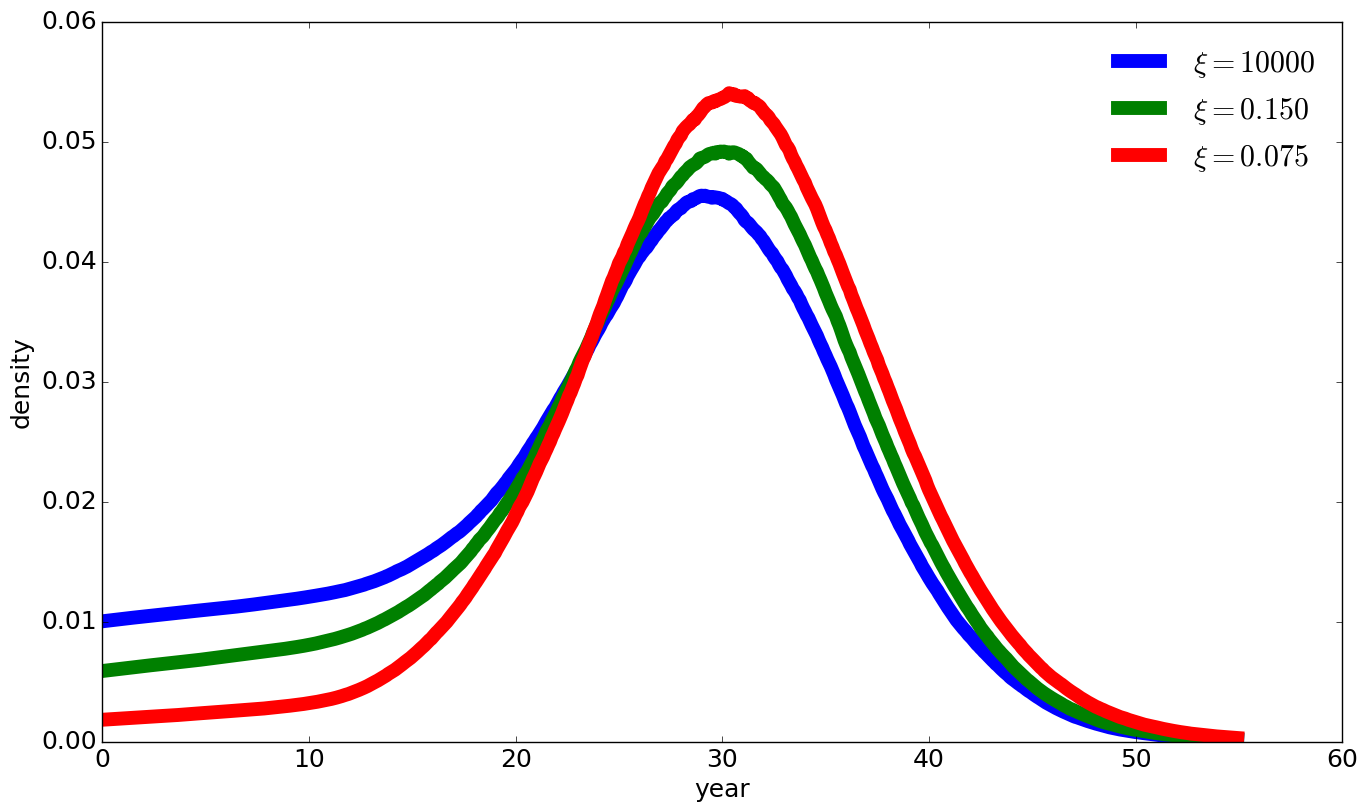
Fig. 3 Densities of first jump, varying with value of \(\xi\)

References

[AHS03]

Evan W Anderson, Lars Peter Hansen, and Thomas J Sargent. A quartet of semigroups for model specification, robustness, prices of risk, and model detection. Journal of the European Economic Association, 1(1):68–123, 2003.

[BBHZ24]

Michael Barnett, William A. Brock, Lars Peter Hansen, and Hong Zhang. Uncertainty, Social Valuation, and Climate Change Policy (Working Paper). 2024.

[BorovivckaHS14]

Jaroslav Borovička, Lars Peter Hansen, and Jose A. Scheinkman. Shock elasticities and impulse responses. Mathematics and Financial Economics, 2014. doi:10.1007/s11579-014-0122-4.

[FLL+99] (1,2,3)

E Fournie, J M Lasry, J Lebuchoux, P L Lions, and N Touzi. Applications of Malliavin calculus to Monte Carlo methods in finance. Finance and Stochastics, 3:391–413, 1999.

Footnotes

---

[1]

Our initial condition for \(\Lambda_0\) differs from [Fournie et al., 1999] in a superficial way. They treat \(\Lambda\) as a matrix with an identity as the initialization. In this way, they consider all of the states of interest simultaneously. We take \(\Lambda\) to be a vector and characterize the marginal initial responses one at a time by letting the initial condition be any one of the coordinate vectors.