7. Likelihoods

This chapter studies likelihood processes and likelihood ratio processes. Derivatives of log-likelihood processes are additive martingales and likelihood ratio processes are multiplicative martingales, assertions that we verify by applying results from chapter Processes with Markovian increments. We study properties of likelihood ratios as sample size \(T \rightarrow +\infty\) and relate them to methods for estimating parameters that pin down a statistical model from within either a discrete set or a manifold of models. These include maximum likelihood, Bayesian, and robust Bayesian methods. A workhorse in this chapter will be the Law of Large Numbers from chapter Stochastic Processes and Laws of Large Numbers that applies in settings in which there are multiple statistical models.

In this chapter, we adopt settings in which state vectors can be inferred perfectly from observations. Chapter Hidden Markov Models studies situations in which some states are hidden and can be inferred only imperfectly.

7.1. Dependent Processes

Suppose that at date \(t+1\) we observe a \(k\) dimensional random vector \(Z_{t+1}\). We calculate various objects while conditioning on a given probability model. We use some of these calculations to explore alternative models. Each alternative model is presumed to imply a probability measure that is measure-preserving and ergodic. An event collection \({\mathfrak A}_t\) (i.e., a sigma algebra) is generated by the infinite history of \(Z_t\).

We entertain a set of alternative probability models represented with their one-period transition probabilities. We represent an alternative model as a perturbation of a baseline model. To represent a particular alternative model, we use a nonnegative random variable \(N_{t+1}\) to perturb a baseline model’s one step transition probabilities. We can characterize an alternative model with a set of implied conditional expectations of all bounded random variable \(B_{t+1}\) that are measurable with respect to \({\mathfrak A}_{t+1}\). Such conditional expectations of \(B_{t+1}\) under the alternative model can be represented as conditional expectations of \(N_{t+1} B_{t+1}\) under the baseline model:

(7.1)\[E \left(N_{{t+1}} B_{{t+1}} \mid {\mathfrak A}_t \right) . \]

Thus, multiplication of \(B_{t+1}\) serves in effect to change the baseline probability from the baseline model to the alternative model. To serve this purpose the random variable \(N_{t+1}\) must satisfy:

1. \(N_{t+1} \ge 0\);

2. \(E\left(N_{t+1} \mid {\mathfrak A}_t \right) = 1\);

3. \(N_{t+1}\) is \({\mathfrak A}_{t+1}\) measurable.

Property 1 is satisfied because conditional expectations map positive random variables \(B_{t+1}\) into positive random variables that are \({\mathfrak A}_t\) measurable. Property 2 is satisfied because conditional expectations of random variables \(B_{t+1}\) that are \({\mathfrak A}_t\) measurable should equal \(B_{t+1}\). Property 3 can be imposed without loss of generality because if it were not satisfied, we could just replace it with \(E \left(N_{t+1} \mid {\mathfrak A}_{t+1} \right)\).

This way of representing an alternative probability model is restrictive. Thus, if a nonnegative random variable has conditional expectation zero under the baseline probability, it will also have zero conditional expectation under the alternative probability measure, a version of absolute continuity here applied to transition probabilities. Violating absolute continuity would make possible model decision rules that correctly select models with full confidence from only finite samples.

Example 7.1

Consider a baseline Markov process having transition probability density \(pi_o\) with respect to a measure \(\lambda\) over the state space \(\mathcal{X}\)

\[P_o(dx^+|x) \lambda(dx^+) = \pi_o(x^+ \mid x) \lambda(dx^+)\]

Let \(\pi\) denote some other transition density that we represent as

\[\pi(x^+ \mid x) \lambda(dx^+ ) = \left[ {\frac {\pi(x^+ \mid x)}{\pi_o(x^+ \mid x)}}\right] \pi_o(x^+ \mid x) \lambda(dx^+ )\]

where we assume that \(\pi_o(x^+ \mid x) = 0\) implies that \(\pi(x^+ \mid x) = 0\) for all \(x^+\) and \(x\) in \(\mathcal{X}\).
Construct the likelihood ratio

\[N_{t+1} = {\frac {\pi(X_{t+1} \mid X_t)}{\pi_o(X_{t+1} \mid X_t)}} .\]

Example 7.2

Suppose that

\[\begin{split}X_{t+1} = {\mathbb A} X_t + {\mathbb B} W_{t+1} \\ Z_{t+1} = {\mathbb D} X_{t} + {\mathbb F} W_{t+1},\end{split}\]

where \({\mathbb A}\) is a stable matrix, \(\{W_{t+1}\}_{t=0}^\infty\) is an i.i.d. sequence of \({\cal N}(0,I)\) random vectors conditioned on \(X_0\), and \({\mathbb F}\) is a nonsingular square matrix. The conditional distribution of \(Z_{t+1}\) is normal with mean \({\mathbb D}X_t\) and nonsingular covariance matrix \({\mathbb F}{\mathbb F}'\). We suppose that \({\mathbb A}\) and \({\mathbb B}\) can be constructed as functions of \({\mathbb D}\) and \({\mathbb F}\).

Since \({\mathbb F}\) is nonsingular, the following recursion connects state and observation vectors:

\[X_{t+1} = \left({\mathbb A} - {\mathbb B}{\mathbb F}^{-1}{\mathbb D} \right)X_t + {\mathbb B} {\mathbb F}^{-1} Z_{t+1}\]

If \(\left({\mathbb A} - {\mathbb B}{\mathbb F}^{-1}{\mathbb D} \right)\) is a stable matrix, we can construct \(X_{t+1}\) as a linear functon of \(Z_{t+1-\tau}\) for \(\tau = 0, 1, \ldots\).

Assume a baseline model that has the same functional form with particular settings of the parameters that appear in the matrices \(({\mathbb A}_o, {\mathbb B}_o, {\mathbb D}_o, {\mathbb F}_o).\) Let \(N_{t+1}\) be the one-period conditional log-likehood ratio

\[\begin{split}\log N_{t+1} = - {\frac 1 2} (Z_{t+1} - {\mathbb D} X_t)'\left({\mathbb F}{\mathbb F}'\right)^{-1}(Z_{t+1} - {\mathbb D} X_t) \\ + {\frac 1 2} \left(Z_{t+1} - {\mathbb D}_o X_t \right)'\left({\mathbb F}_o{{\mathbb F}_o}'\right)^{-1} \left(Z_{t+1} - {\mathbb D}_o X_t \right) \\ - {\frac 1 2} \log \det \left({\mathbb F}{\mathbb F}'\right) + {\frac 1 2} \log \det \left( {\mathbb F}_o{{\mathbb F}_o}'\right)\end{split}\]

Notice how we have subtracted components coming from the baseline model.

7.2. Likelihood Ratio Processes

The random variable \(N_{t+1}\) contains the new information in observation \(Z_{t+1}\) that is relevant for comparing an alternative statistical model to a baseline model. As data arrive, information accumulates in a way that we describe by compounding the process \(\{N_{t+1} : t \ge 0\}\):

\[L_{t+1} = \prod_{j=0}^{t} N_{j+1}\]

so that

\[\log L_{t+1} = \sum_{j=0}^t \log N_{j+1}\]

Being functions of a stochastic process of observations \(\{Z_{t+1} : t\ge 0 \}\), the likelihood ratio and log-likelihood ratios sequences are both stochastic processes.

Fact 6.1 Since \(E \left( N_{t+1} \mid {\mathfrak A}_t \right) = 1\), a likelihood ratio process satisfies

\[E \left( L_{t+1} \mid {\mathfrak A}_t \right) = L_t .\]

Therefore, it is a martingale relative to the information sequence \(\{ {\mathfrak A}_t : t\ge 0\}\)

Fact 6.2 A log-likelihood ratio process \(\left\{ \log(L_{t+1}) : t=0,1,\ldots,t\right\}\) is a stationary increment process with increment

\[\log L_{t+1}- \log L_t = \log N_{t+1}.\]

The log-likelihood process is additive in how it accumulates stationary increments \(\log N_{t+1}\). Consequently, the likelihood ratio process is what we call a multiplicative process.

Our next fact uses Jensen’s inequality for the concave function \(\log (N)\) illustrated in fig:jensen.

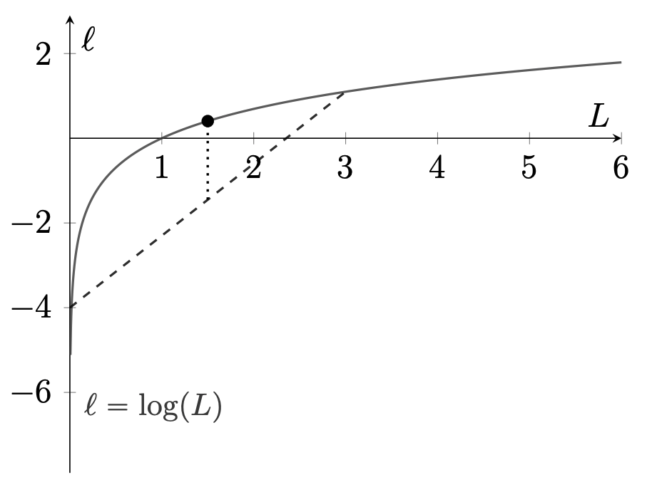
Fig. 7.1 Jensen’s Inequality. The logarithmic function is the concave function that equals zero when evaluated at unity. An interior average of the endpoints of the straight line lies below the logarithmic function. Jensen’s Inequality asserts that the line segment lies below the logarithmic function.

Fact 6.3 By Jensen’s inequality,

\[E \left(\log N_{t+1} \mid {\mathfrak A}_t \right) \le \log E \left(N_{t+1} \mid {\mathfrak A}_t \right) = 0,\]

where the mathematical expectation is again under the baseline model parameterized by \(\theta_o\). Thus

\[E \left(\log L_{t+1} \mid {\mathfrak A}_t \right) \le \log L_t.\]

This implies that under the baseline model the log-likelihood ratio process is a super martingale relative to the information sequence \(\{ {\mathfrak A}_t : t\ge 0\}\).

Notice that if \(N_{t+1}\) is not identically one, then

\[E \left(\log N_{t+1} \right) < 0.\]

From the Law of Large Numbers, the population mean is well approximated by a sample average from a long time series. That opens the door to discriminating between two models. Under the baseline model, the log likelihood ratio process scaled by the inverse of the sample size \(t+1\) converges to a negative number. After changing roles of the baseline and alternative models, we can do an analogous calculation that entails using \({\frac 1 {N_{t+1}} }\) instead of \(N_{t+1}\) as an increment. Then the scaled-by-\((t+1)^{-1}\) log likelihood ratio would converge to the expectation of \(- \log N_{t+1}\) under the alternative model that is now in the denominator of the likelihood ratio. This limit would be positive under the assumption that the alternative model generated the data. These calculations justify selecting between the two models by calculating \(\log L_{t+1}\) and checking if it is positive or negative. This procedure amounts to a special case of the method of maximum likelihood.

Remark 7.1

Suppose that data are not generated by the baseline model. Instead, suppose that the statistical model implied by the change of measure \(N_{t+1}\) governs the stochastic evolution of the observations. Define conditional entropy relative to baseline model \(\theta_o\) as the following conditional expectation:

\[E \left( N_{t+1} \log N_{t+1} \mid {\mathfrak A}_t \right).\]

Here multiplication of \(\log N_{t+1}\) by \(N_{t+1}\) changes the conditional probability distribution from the misspecified baseline model to the alternative statistical model that we assume generates the data. The function \( n \log n\) is convex and equal to zero for \(n=1\). Therefore, Jensen’s inequality implies that conditional relative entropy is nonnegative and equal to zero when \(N_{t+1} = 1\). An unconditional counterpart of relative entropy is the Law of Large Numbers limit

\[\lim_{t \rightarrow +\infty} {\frac 1 {t+1} } \sum_{j=0}^t \log N_{t+1} = \lim_{t \rightarrow + \infty} {\frac 1 {t+1} } \sum_{j=0}^t E \left(N_{t+1} \log N_{t+1} \mid {\mathfrak A}_t \right) \ge 0\]

under the data generating process. Relative entropy is often used to analyze model misspecifications. It is also a key component for studying the statistical theory of “large deviations” for Markov processes, as we shall discuss later.

7.2.1. Bayes’ law and likelihood ratio processes

Suppose now that we attach a prior probability \(\pi_o\) to the baseline model with probability \(1 - \pi_o\) on the alternative. Then after observing \(Z_{j+1}: 0 \le j \le t\), conditional probabilities for the baseline and alternative models are

\[{\frac {\pi_o}{L_{t+1} (1-\pi_o) + \pi_o}} \quad {\textrm{and}} \quad \frac {L_{t+1}(1 - \pi_o)}{L_{t+1} (1-\pi_o) + \pi_o} .\]

When \({\frac 1 {t+1}} \log L_{t+1}\) converges to a negative number, the first probability converges to one, and when \({\frac 1 {t+1}} \log L_{t+1}\) converges to a positive number, it converges to zero.

7.3. Parameterizing Likelihoods

Let \( \Theta \) be a set of parameter vectors. Each \( \theta \in \Theta \) indexes an alternative transition probability as represented by the \( N_{t+1}(\theta) \) that belongs in formula (7.1). We presume that a particular \( \theta \), denoted \( \theta_o \), indexes the transition probability that generates the data and is used as to calculate the conditional expectation in formula (7.1). Accordingly, \( N_{t+1}(\theta_o) = 1 \). Since \( N_{t+1}(\theta) \) is a likelihood increment, a recursion that defines a likelihood ratio process for each \( \theta \) is

\[L_{t+1} (\theta) = N_{t+1}(\theta) L_t(\theta) \]

Setting \( L_0(\theta) = 1 \) for each \( \theta \) completes a parameterized family of likelihood ratios.

But the applied researcher does not know \( \theta_o \). For that reason, it is convenient now to use a model with some arbitrary known parameter vector \( {\tilde \theta} \in \Theta \) as a baseline model in place of the \( \theta_o \) model. We can accomplish this by defining an increment process \( \widetilde N_{t+1}(\theta) \) as

\[{\widetilde N}_{t+1}(\theta) = {\frac {N_{t+1}(\theta) }{ N_{t+1}(\tilde \theta)}} .\]

Notice that when we use \( {\widetilde N}_{t+1}(\theta) \) in formula (7.1), we must also change the transition probability used to take the expectation in (7.1) to be the transition probability implied by \( {\tilde \theta} \). This is evident because \( {\widetilde N}_{t+1}(\tilde \theta) = 1 \). Our change of baseline model leads us now to construct likelihood ratios with the recursion:

\[{\widetilde L}_{t+1} (\theta) = {\widetilde N}_{t+1}(\theta) {\widetilde L} _t( \theta),\]

where we set \( {\widetilde L}_0(\theta) = 1 \). In this way, we construct parameterized likelihoods without knowing the \( \theta_o \) model that generates the data.

In order to apply the Law of Large Numbers to the logarithm of the likelihood ratio process divided by \( t+1 \), namely to

\[{\frac 1 {t+1}} \log {\widetilde L}_{t+1}(\theta) = {\frac 1 {t+1}} \sum_{j=0}^{t} \log {\widetilde N}_{j+1} (\theta)\]

for \( t \ge 0 \), we want to compute expectations under the \( \theta_o \) model that actually generates the data. Under the \( \theta_o \) model’s expectation operator

\[{\tilde \nu}(\theta) = E \left[ \log {\widetilde N}_{t+1}(\theta) \right] = E \left[ \log { N}_{t+1}(\theta) \right] - E \left[ \log { N}_{t+1}(\tilde \theta) \right] = \nu(\theta) - \nu( {\tilde \theta}) .\]

7.3.1. Maximum Likelihood

We want the law of large numbers from chapter Stochastic Processes and Laws of Large Numbers eventually to disclose the parameter vector \( \theta_o \). The following argument shows that it will. The law of large numbers leads us to expect that

\[\lim_{t \rightarrow + \infty} \frac{1 }{1 +t} \log {\widetilde L}_{t+1} = {\tilde \nu}(\theta) .\]

Since \( \theta_o \) generates the data, the super martingale property of the log likelihood ratio process implies that

\[\nu(\theta) \le \nu(\theta_o) = 0. \]

Therefore

\[ {\tilde \nu}(\theta) = \nu(\theta) -\nu(\tilde \theta) \le \nu(\theta_o) - \nu(\tilde \theta) = \tilde \nu(\theta_o) .\]

This implies that \( \theta_o \) is a maximizer of \( \tilde \nu(\theta) \), and gives a “population counterpart” to maximum likelihood estimation. By a population counterpart, we imagine a setting in which via the law of large numbers, sample averages have converged to their population counterparts. Formally, a population counterpart to maximum likelihood estimation solves:

\[\max_{\theta \in \Theta} {\tilde \nu}(\theta) .\]

We have shown that the set of \( \theta \)‘s that solve \( \max_{\theta \in \Theta} \nu(\theta) \) includes \( \theta_o \). We say that the model is identified if \( \theta_o \) is the unique maximizer. The maximum likelihood estimator from a finite data sample uses a sample counterpart of the above equation, namely,

\[{\textrm{ argmax}}_{\theta \in \Theta} {\frac 1 {t+1}} \log {\widetilde L}_{t+1} (\theta) .\]

Remark 7.2

(Reverse relative entropy) Continuing to index conditional distributions by parameter vectors \(\theta \in \Theta\), form the ratio

\[N_{t+1}^o(\theta) = {\frac {{\widetilde N}_{t+1}(\theta_o)}{{\widetilde N} _{t+1}(\theta)}} \]

Using a version of formula (7.1), we can use this ratio of likelihood increments to represent the transition distribution for statistical model \(\theta_o\) relative to that for an arbitrary statistical model \(\theta\). The ratio of likelihood increments effectively changes the baseline model from \(\tilde \theta\) to an arbitrary \(\theta\).
Then the associated unconditional relative entropy defined in Remark 7.1 becomes

\[D(\theta) = \lim_{t \rightarrow +\infty} {\frac 1 {t+1} } \sum_{j=0}^t \log N_{t+1}^o(\theta) \ge 0\]

where the \(\theta_o\) model generates the data. We can then express the population counterpart to maximum likelihood as the solution to a minimum relative entropy problem.
Thus, since the model indexed by parameter vector \(\theta_o\) generates the data, the population maximum likelihood estimator solves

\[\min_{\theta \in \Theta} D(\theta) = 0 .\]

7.4. Score Process

We assume that the parameter vector \(\theta_o\) in the interior of a parameter space \(\Theta\). Moreover, for each \(\theta \in \Theta\),

\[E \left(N_{t+1}(\theta) \mid {\mathfrak A}_t \right) = 1\]

where \(N_{t+1}(\theta_o) = 1\) by construction. Provided that we can differentiate inside the mathematical expectation:[1]

\[E \left( {\frac {\partial N_{t+1}}{\partial \theta}} \Bigl|_{\theta = \theta_o} \mid {\mathfrak A}_t \right) = 0.\]

Since expectations are taken under the \(\theta_o\) probability

\[{\frac {\partial N_{t+1}}{\partial \theta}} \Bigl|_{\theta = \theta_o} = {\frac {\partial \log N_{t+1}}{\partial \theta}} \Bigl|_{\theta = \theta_o}\]

Since the right side is a logarithmic derivative

\[{\frac {\partial \log N_{t+1}}{\partial \theta}} \Bigl|_{\theta = \theta_o} = {\frac {\partial \log {\widetilde N}_{t+1}}{\partial \theta}} \Bigl|_{\theta = \theta_o}\]

where we used \({\widetilde N}_{t+1} (\theta)\) to build an operational likelihood process for alternative \(\theta \in \Theta\).

Definition 7.1

The score increment is

\[S_{t+1} - S_t = {\frac {\partial \log N_{t+1}}{\partial \theta}} \Big|_{\theta = \theta_o}\]

and the score process is

\[S_{t+1} = \frac \partial {\partial \theta} \log L_{t+1} \Big|_{\theta = \theta_o} \]

Fact 6.4 The score process \(\{S_{t+1} : t \ge 0\}\) is a (multivariate) martingale with stationary increments. Consequently

\[\frac 1 {\sqrt{t}} S_{t+1} \Rightarrow {\mathcal N}(0, {\mathbb V})\]

where \({\mathbb V} = E \left[ \left( S_{t+1} - S_t \right) \left( S_{t+1} - S_t \right)' \right]\).

Fact 6.4 motivates characterizing the large sample behavior of the score process by utilizing the martingale central limit theorem stated in Proposition 3.2. In effect, the matrix \({\mathbb V}\) measures curvature of the log-likelihood process in the neighborhood of the “true” parameter value \(\theta_o\). The more curvature there is – i.e., the “larger” is the variance matrix \({\mathbb V}\) of the score vector – the more information the data contain about \(\theta\). The matrix \({\mathbb V}\) is called the Fisher information matrix in honor of R.A. Fisher.

An associated central limit approximation yields a large sample characterization of the maximum likelihood estimator of \(\theta\) in a Markov setting. Let \(\theta_t\) maximize the log-likelihood function \(\log L_t(\theta)\). Under some regularity conditions

\[\sqrt{t} (\theta_t - \theta_o ) \rightarrow {\mathcal N}\left(0, {\mathbb V}^{-1}\right).\]

This limit justifies interpreting the covariance matrix \({\mathbb V}\) of the martingale increment of the score process as quantifying information that data contain about the parameter vector \(\theta_o\).

7.5. Nuisance parameters

Consider a situation in which to learn about one parameter, we have to estimate other parameters too. Suppose that \(\theta\) is a vector and \(\mathbb{V}\) is a matrix. We seek a notion of “Fisher information” about a single component of \(\theta\) that interests us – a single parameter \(\bar{\theta}\). A natural guess might be simply to take as our measure the appropriate diagonal entry of \(\mathbb{V}\). It turns out that this measure of our uncertainty is misleading because it ignores the fact that in order to estimate the parameter of interest to us we have to “spend” some of the information in the sample to estimate “nuisance parameters” that we also had to estimate in order make inferences about \(\bar{\theta}\). It turns out that a better way to summarize our uncertainty about the parameter of interest is to define its “Fisher information” as the reciprocal of an appropriate entry of \(\mathbb{V}^{-1}\).

Thus, partition

\[\begin{split}\theta = \begin{bmatrix} {\bar{\theta}} \\ {\tilde{\theta}} \end{bmatrix}\end{split}\]

where \(\bar{\theta}\) is the scalar parameter of interest and \(\tilde{\theta}\) is an associated unknown nuisance parameter vector.

Write the multivariate score process as

\[\begin{split}\left\{ \begin{bmatrix} {\overline{S}_{t+1}} \\ {\widetilde{S}}_{t+1} \end{bmatrix} : t=0,1,... \right\}\end{split}\]

Partition the covariance matrix \(\mathbb{V}\) of the score process increment conformably with \((\bar{\theta}', {\tilde{\theta}}')'\):

\[\begin{split}\begin{bmatrix} E\left({\overline{S}}_{t+1} - {\overline{S}}_t \right)^2 & E \left({\overline{S}}_{t+1} - {\overline{S}} _t \right)\left(\widetilde{S}_{t+1} - \widetilde{S}_t \right)' \\ E \left(\widetilde{S}_{t+1} - \widetilde{S}_t \right)\left({\overline{S}}_{t+1} - {\overline{S}}_t \right) & E \left(\widetilde{S}_{t+1} - \widetilde{S}_t\right) \left(\widetilde{S}_{t+1} - \widetilde{S}_t\right) ' \end{bmatrix} \equiv \begin{bmatrix} {\mathbb{V}}_{11} & {\mathbb{V}}_{12} \\ {\mathbb{V}}_{21} & {\mathbb{V}}_{22} \end{bmatrix}.\end{split}\]

We claim that taking \(E\left({\overline{S}}_{t+1} - {\overline{S}}_t \right)^2 \) as a measure of “Fisher information” about \(\bar{\theta}\) would overstate our information. Instead, the appropriate Fisher information about \(\bar{\theta}\) is the inverse of the \((1,1)\) component of the asymptotic covariance matrix \(\mathbb{V}^{-1}\). Applying a partitioned inverse formula for a symmetric matrix to compute that measure of Fisher information yields

(7.2)\[I_{\bar{\theta}} = {\mathbb{V}}_{11} - {\mathbb{V}}_{12} {\mathbb{V}}_{22}^{-1} {\mathbb{V}}_{12}'.\]

An enlightening interpretation of the \((1,1)\) component \(I_{\bar{\theta}}\) of \(\mathbb{V}^{-1}\) comes from recognizing that it is the residual variance of a population least squares regression of the score vector increment of \(\bar{\theta}\) on the score vector increment for the nuisance parameter vector \(\widetilde{\theta}\).

Thus, a population least squares regression is

(7.3)\[{\overline{S}}_{t+1} - {\overline{S}}_t = \beta ({\widetilde{S}}_{t+1} - {\widetilde{S}}_t) + U_{t+1},\]

where \(\beta\) is a population regression coefficient vector and \(U_{t+1}\) is a population regression residual that by construction is orthogonal to the regressor \(({\widetilde{S}}_{t+1} - {\widetilde{S}}_t)\). The least squares regression coefficient vector is

\[\beta = {\mathbb{V}}_{12} {\mathbb{V}}_{22}^{-1}\]

and the residual variance is

\[E U_{t+1}^2 = {\mathbb{V}}_{11} - {\mathbb{V}}_{12} {\mathbb{V}}_{22}^{-1} {\mathbb{V}}_{12}'\]

which equals the Fisher information measure \(I_{\bar{\theta}}\) defined above. From the orthogonality of least squares residuals to regressors, the variability of the left side variable \({\overline{S}}_{t+1} - {\overline{S}}_t\) in the projection equation (7.3) cannot exceed that of the least squares residual so that

\[E (U_{t+1})^2 \le E \left({\overline{S}}_{t+1} - {\overline{S}}_t\right)^2,\]

an inequality that confirms that information about \(\bar{\theta}\) is lost by not knowing the nuisance parameters \(\tilde{\theta}\).

---

[1]

Formally, we define the derivative of a family \(\{ \log N_{t+1}(\theta) : \theta \in \Theta\}\) in terms of mean square limits, and we let \({\frac {\partial N_{t+1}}{\partial \theta}}= N_{t+1} {\frac {\partial N_{t+1}}{\partial \theta}}\).