10. Representing Marginal Valuation

Authors: Lars Peter Hansen and Thomas J. Sargent

Date: November 2024 \(\newcommand{\eqdef}{\stackrel{\text{def}}{=}}\)

10.1. Introduction

Partial derivatives of value functions appear in first-order conditions of Markov decision problems and measure marginal valuations. Since controls depend on partial derivatives of value functions, they also feature prominently in max-min formulations of robust control problems. They can also be used to measure losses from suboptimal choices. They are pertinent for both individual decision problems and social evaluations. Robust control theories have been used by [Hansen et al., 1999] to assess impacts of uncertainty on investment and equilibrium prices and quantities, by [Alvarez and Jermann, 2004] to evaluate the welfare consequences of uncertainty, and by [Barnett et al., 2020] to characterize social costs of carbon emissions in the presence of uncertainty about damages inflicted by climate changes. Social costs of global warming are important contributors to social costs of carbon emissions that are often inferred from marginal impacts of fossil fuel emissions on climate indicators. These depend on uncertain damages to future economic opportunities.

This chapter imports insights about stochastic nonlinear impulse response functions that come from asset pricing methods for valuing uncertain cash flows. Our analysis relies on decompositions of partial derivatives that allow researchers to partition quantitative findings into contributing forces. This approach contributes to a broader agenda that aims to improve uncertainty quantification methods. Dynamic stochastic equilibrium models often involve several moving parts. Decomposing sources of implications from such models ``opens black boxes’’ In markdown it is better to use double quotation marks “”. I have changed this elsewhere and helps provide plausible explanations of model outcomes. Our asset-pricing perspective allows us to think in terms of state-dependent discounting and stochastic flows reminiscent of stochastic payoffs to be valued. Moreover, this perspective allows us to relate stochastic flow to forcing functions that drive outcomes a dynamic stochastic equilibrium model.

10.2. Discrete time

We start with Markov process

(10.1)\[\begin{split}X_{t+1} = \psi(X_t, W_{t+1}) \\ Y_{t+1} - Y_t = \kappa(X_t, W_{t+1}),\end{split}\]

with \(n\) components of \(X,\) \(Y\) a scalar, and \(W\) is \(k\) dimensional. We also want to study the associated variational processes

(10.2)\[\begin{split}\Lambda_{t+1} = \frac {\partial \psi}{\partial x'} (X_t, W_{t+1}) \Lambda_t \\ \Delta_{t+1} - \Delta_t = \frac {\partial \kappa}{\partial x}(X_t, W_{t+1}) \cdot \Lambda_t .\end{split}\]

We use stochastic impulse responses to provide an “asset pricing” representation of partial derivatives of a value function with respect to one of the components of \(X_0\). Consider a value function that satisfies:

(10.3)\[\begin{split}\begin{align} V(X_t) + Y_t = & \exp(-\delta) \mathbb{E} \left[ V(X_{t+1}) + Y_{t+1} \mid X_t \right] \\ & + [1 - \exp(-\delta)] \left[ U(X_t) + Y_t \right]. \end{align}\end{split}\]

As I brought up in the email, maybe it would be beneficial to readers a sentence or two explaining why this particular form of value function is worth studying, although perhaps this is obvious to readers with more awareness of the literature than me. This value function might measure outcomes from using some arbitrary collection of decision rules, not necessarily socially optimal ones. To do a local policy analysis, we’ll want to compute marginal valuations for such a value function.

Differentiate both sides of this (10.3) with respect to \(X_t\) and \(Y_t\) and form dot products with appropriate variational counterparts:

(10.4)\[\begin{split}\begin{align} \frac{\partial V}{\partial x}(X_t) \cdot \Lambda_t + \Delta_t = & \exp(-\delta) \mathbb{E}\left[ \frac{\partial V}{\partial x}(X_{t+1}) \cdot \Lambda_{t+1} + \Delta_{t+1} \mid X_t, \Lambda_t, \Delta_t \right] \\ & + [1 - \exp(-\delta)]\left[\frac{\partial U}{\partial x}(X_t) \cdot \Lambda_t + \Delta_t \right] \end{align} \end{split}\]

View equation (10.4) as a stochastic difference equation and solve it forward for \(\frac{\partial V}{\partial x}(X_t) \cdot \Lambda_t + \Delta_t:\)

(10.5)\[\begin{align*} & \frac{\partial V}{\partial x}(X_t) \cdot \Lambda_t + \Delta_t = \cr & [1 - \exp(-\delta)]\sum_{\tau = 0}^\infty \mathbb{E}\left( \exp(-\tau \delta) \left[\frac{\partial U}{\partial x}(X_{t+\tau}) \cdot \Lambda_{t+\tau} + \Delta_{t + \tau}\right] \mid X_t, \Lambda_t, \Delta_t \right) \end{align*}\]

Initialize \(\Lambda_0 = \mathrm{e}_i,\) where \(\mathrm{e}_i\) is a coordinate vector with a one in position \(i\) and \(\Delta_0 = 0.\) This lets us represent the partial derivative of the value function as:

\[\begin{align} & \frac{\partial V}{\partial x_i}(x) = \cr & [1 - \exp(-\delta)]\sum_{t = 0}^\infty \exp(-t \delta) \mathbb{E}\left[ \frac{\partial U}{\partial x}(X_{t}) \cdot \Lambda_{t} + \Delta_t \mid X_0 = x, \Lambda_0 = \mathrm{e}_i, \Delta_0 = 0 \right] , \end{align} \]

which resembles an asset pricing formula in which

\[\begin{split}\left\{\exp(-\delta t)\begin{bmatrix} \Lambda_t \\ \Delta_t \end{bmatrix} : t \ge 0 \right\}\end{split}\]

acts as a vector stochastic discount factor process Maybe I misunderstood but shouldn’t the second entry of the cash flow vector be 1 instead of \(\Delta_t\)? and the marginal contribution

\[\begin{split}\left\{ [1 - \exp(-\delta)]\begin{bmatrix} \frac{\partial U}{\partial x}(X_{t}) \\ \Delta_t \end{bmatrix} : t \ge 0\right\},\end{split}\]

acts as a vector stochastic cash flow process. The stochastic impulse response tells the marginal response of state vector at date \(t\) to changes in the \(i^{th}\) state vector component at date zero, while the vector of marginal cash flows at date \(t\) measures impacts on utility of a marginal change in the date \(t\) state vector.

Remark 10.1

Sometimes it is convenient to apply summation by parts:

\[\begin{split}\begin{align*} & [1 - \exp(-\delta)]\sum_{\tau = 0}^\infty \mathbb{E}\left( \exp(-\tau \delta) \Delta_{t + \tau} \mid X_t, \Lambda_t, \Delta_t \right) \\ & = \sum_{\tau = 1}^\infty \mathbb{E}\left[ \exp(-\tau \delta) \left(\Delta_{t + \tau} - \Delta_{t+\tau -1} \right) \mid X_t, \Lambda_t, \Delta_t \right] + \Delta_t \\ & = \sum_{\tau = 1}^\infty \mathbb{E}\left[ \exp(-\tau \delta) \frac{\partial \kappa}{\partial x}(X_{t+\tau-1}, W_{t+\tau})\cdot \Lambda_{t+ \tau} \mid X_t, \Lambda_t, \right] + \Delta_t . \end{align*}\end{split}\]

Substituting into (10.5) gives:

\[\begin{split}\begin{align} &\frac{\partial V}{\partial x}(X_t) \cdot \Lambda_t + \Delta_t = \cr & [1 - \exp(-\delta)]\sum_{\tau = 0}^\infty \mathbb{E}\left[ \exp(-\tau \delta) \frac{\partial U}{\partial x}(X_{t+\tau}) \cdot \Lambda_{t+\tau} \mid X_t, \Lambda_t, \right] \\ & + \sum_{\tau = 1}^\infty \mathbb{E}\left[ \exp(-\tau \delta) \frac{\partial \kappa}{\partial x}(X_{t+\tau-1}, W_{t+\tau})\cdot \Lambda_{t+ \tau} \mid X_t, \Lambda_t, \right] + \Delta_t. \end{align}\end{split}\]

10.3. Continuous time

A continuous-time formulation allows us to distinguish small shocks (Brownian increments) from large shocks (Poisson jumps). Let’s consider a continuous-time specification with Brown motion shocks, i.e., diffusion dynamics. We can treat jumps as terminal conditions for which we impose continuation values conditioned on a jump taking place. The possibility of a jump contributes to the value function. After developing this approach, we shall extend it to we include valuations that reflect concerns about model misspecifications, i.e., “robust valuations.”

10.3.1. Diffusion dynamics

We start with a Markov diffusion that governs state dynamics

\[\begin{split}\begin{align*} dX_t & = \mu(X_t) dt + \sigma(X_t) dW_t \\ dY_t & = \nu(X_t) dt + \varsigma(X_t) \cdot dW_t. \end{align*}\end{split}\]

that need not be the outcome of an optimization problem.

Using the variational process construction in the previous chapter, recall that

\[d\Lambda_{t}^i = \left(\Lambda_t\right)'\frac{\partial \mu_i}{\partial x}(X_t) dt + \left({\Lambda_t}\right)'\frac{\partial \sigma_i}{\partial x}(X_t) dW_t.\]

With the appropriate stacking, the drift for the composite process \((X,\Lambda)\) is:

(10.6)\[\begin{split}\mu^a(x,\lambda) \overset{\text{def}}{=} \begin{bmatrix} \mu(x) \\ \lambda'{\frac {\partial \mu_i} {\partial x} }(x) \\ ... \\ \lambda'{\frac {\partial \mu_n} {\partial x} }(x) \end{bmatrix},\end{split}\]

and the composite matrix coefficient on \(dW_t\) is given by

(10.7)\[\begin{split}\sigma^a(x,\lambda) \overset{\text{def}}{=} \begin{bmatrix} \sigma(x) \\ \lambda'\frac {\partial \sigma_1 }{\partial x}(x)\\ ... \\ \lambda' \frac {\partial \sigma_n }{\partial x}(x) \end{bmatrix}.\end{split}\]

Similarly, \(\Delta\) is the scalar variational process associated with \(Y\) with evolution

\[d \Delta_t = \Lambda_t \cdot \frac {\partial \nu}{\partial x} (X_t)dt + {\Lambda_t}' \frac {\partial \varsigma}{\partial x'} dW_t \]

10.3.2. An initial representation of a partial derivative

Consider the evaluation of discounted utility where the instantaneous contribution is \(U(x)\) where \(x\) is the realization of a state vector \(X_t\). The function \(U\) satisfies a Feynman-Kac (FK) equation:

(10.8)\[\begin{align} 0 = & \delta \left[U(x) + y\right] - \delta \left[V(x) + y \right] + \mu(x) \cdot \frac {\partial V}{\partial x}(x) + \nu(x) \cr &+ {\frac 1 2 }{\rm trace}\left[\sigma(x)' \frac {\partial^2 V}{\partial x \partial x'}(x) \sigma(x) \right]. \end{align}\]

As in the discrete-time example, we want to represent

\[V_{x_i}(x) = {\frac {\partial V}{\partial x_i}}(x) \]

as an expected discounted value of a marginal impulse response of future \(X_t\) to a marginal change of the \(i^{th}\) coordinate of \(x.\)

By differentiating Feynman-Kac equation (10.8) with respect to each coordinate, we obtain a vector of equations, one for each state variable. We then form the dot product of this vector system with respect to \(m\) to obtain a scalar equation system that is of particular interest. What is \(m\)? Should it be \(\lambda\)?The resulting equation is a Feynman-Kac equation for the scalar function:

\[\lambda \cdot \frac {\partial V}{\partial x}\]

as established in the Appendix. Given that the equation to be solved involves both \(\lambda\) and \(x\), this equation uses the diffusion dynamics for the joint process \((X,\Lambda)\).

The solution to this Feynman-Kac equation takes the form of a discounted expected value:

(10.9)\[\begin{align} & \frac {\partial V}{\partial x}(X_0) \cdot \Lambda_0 + \Delta_0 \cr &= \delta \int_0^\infty \exp( - \delta t ) {\mathbb E} \left[ \frac {\partial U}{\partial x} (X_{t}) \cdot \Lambda_{t} + \Delta_t \mid X_0, \Lambda_0, \Delta_0 \right] dt. \end{align} \]

By initializing the state vector \(\Lambda_0\) to be a coordinate vector of zeros in all entries except \(i\) and \(\Lambda_0 = 0\), we obtain the formula we want, which gives the partial derivative as a discounted present value using \(\delta\) as the discount rate. The contribution, \(\Lambda_{t},\) is the marginal response of the date \(t\) state vector to marginal change in the \(i^{th}\) component of the state vector at date zero. The marginal change in the date \(t\) state vector induces marginal reward at date \(t\):

\[\delta \frac {\partial U}{\partial x} (X_{t})\cdot \Lambda_{t} + \Delta_t\]

which provides us with a useful interpretation as an asset price. The process \(\Lambda\) gives a vector counterpart to a stochastic discount factor process and \(\delta \frac {\partial U}{\partial x} (X_{t}) + \Delta_t\) gives the counterpart to a cash flow to be valued.

One application of representation (10.9) computes the discounted impulse response:

\[\delta \exp( - \delta t ) {\mathbb E} \left[ \frac {\partial U}{\partial x_j} (X_{t}) \cdot \Lambda_{t} \mid X_0, \Lambda_0, \Delta_0 \right]. \]

for \(t \ge 0\) and for \(j=1,2,...,n\) along with

\[\delta \exp( - \delta t ) {\mathbb E} \left[ \Delta_t \mid X_0, \Lambda_0, \Delta_0 \right] \]

for \(t \ge 0\) as an intertemporal, additive decomposition of the marginal valuation of one of the state variables as determined by an initialization of \(\Lambda_0.\)

Remark 10.2

Representations similar to (10.7) appear in the sensitivity analyses of options prices. See [Fournie et al., 1999].

10.3.3. Robustness

We next consider a general class of drift distortions that can help us study model misspecification concerns. We initially explore the consequences of exogenously-specified drift distortion. After that, we show how such a distortion can emerge endogenously as a decision-maker’s response to concerns about model misspecifications.

For diffusions, we entertain distortions to the Brownian increment. Instead \(W\) being a multivariate Brownian motion, we allow it to have a drift \(H\) under a change in the probability distribution. We index the alternative probability specifications with their corresponding drift processes \(H\). Locally,

\[dW_t = H_t dt + dW^H_t\]

where \(W^H\) is a Brownian motion under the \(H\) probability. Given that both the distribution parameterized by \(H\) and the baseline distribution for the increment are normals with an identity matrix as the local covariance matrix, the local measure of relative entropy is given by the quadratic term:

\[{\frac 1 2} H_t \cdot H_t .\]

See [James, 1992], [Anderson et al., 2003], and [Hansen et al., 2006] for further discussions.

We pose the decision problem as a Stackelberg game solved from a date zero perspective. The maximizing decision maker takes as given, a drift distortion process, \(\{H_t : t \ge 0 \},\) when optimizing by choice of a decision process \(\{D_t : t \ge 0\}\). The minimizing decision maker then optimizes by choice \(H\). This solution is posed in the space of stochastic processes.

We analyze this problem following on insights in [Fleming and Souganidis, 1989]. They justify a value function, \(V,\) that solves:

(10.10)\[\begin{align} 0 &= \min_h \max_{d \in {\mathcal D} } \hspace{.2cm} \delta\left[ U(x,d) + y\right] - \delta \left[ V(x) + y \right]+ {\frac \xi 2}|h|^2 \cr & + \left[\mu(x,d) +\sigma(x,d)h \right] V_x(x) + \nu(x) + \varsigma(x) \cdot h \cr & + {\frac 1 2} {\rm trace} \left[ \sigma (x,d)' V_{xx}(x) \sigma(x,d) \right]. \end{align}\]

Notice that this value function is constructed by solving a recursive version of the zero-sum game.
One of the conditions they impose is called the Bellman-Isaacs equation requiring the exchanging orders of \(\min\) and \(\max\) does not alter the value function for the recursive game Maybe: One of the conditions they impose is called the Bellman-Isaacs equation, which requires that exchanging the order of \(\min\) and \(\max\) does not alter the value function for the recursive game. In effect, [Fleming and Souganidis, 1989] show that coupled dynamic programs characterize the two-player, zero-sum game that interests us, as well as some other two-player, zero-sum games.

Following [Hansen et al., 2006], this approach gives us a recipe for constructing a minimizing drift distortion process \(\{H_t : t \ge 0\}\). The minimizing \(h\) in (10.10) expressed as a function of \(x\) satisfies:

(10.11)\[h^*(x) = - \frac 1 \xi \left( \sigma'[x, d^*(x)] V_x(x) + \varsigma(x) \right)\]

where \(d^*\) is maximizing \(d.\) Define the drift distortion:

\[H_t^* \eqdef h^*\left({\overline X}_t \right).\]

Would it be clearer to define \({\overline X}_t\) here? Form

\[d \overline{X}_t = {\bar \mu}\left( \overline{X}_t \right) dt + {\bar \sigma} \left({\overline X}_t\right) dW_t^{H^*}\]

and

\[\begin{align*} {\bar \mu}\left( \overline{X}_t \right) \eqdef & \mu\left[ {\overline X}_t, d^*\left( {\overline X}_t \right) \right] + {\bar \sigma} \left({\overline X}_t\right) h^*\left( {\overline X}_t\right) \cr {\bar \sigma} \left({\overline X}_t\right) = & \sigma\left[ {\overline X}_t, d^*\left( {\overline X}_t \right) \right] \end{align*}\]

for the initialization \({\overline X}_0 = X_0\). Given this initial condition, by design \(X_t = {\overline X}_t\) for \(t \ge 0\) is a maximizer for \(\{ D_t : t \ge 0\}.\) We constructed the process \(\{ {\overline X}_t : t \ge 0 \}\) for the sole purpose of representing the minimizing drift distortion.

The maximizing decision maker takes \(\{ {\overline X}_t : t \ge 0\}\) as exogenous when optimizing. We write the stochastic dynamics for the original state vector as:

\[d X_t = \mu(X_t, D_t)dt + \sigma(X_t, D_t) h^* \left( \overline{X}_t \right) dt + \sigma(X_t, d_t ) dW_t^{H^*}.\]

The HJB equation for the maximizing decision maker (taking the minimizing solution as given) is:

(10.12)\[\begin{align} 0 = \hspace{.2cm} & \max_{d \in {\mathcal D}} \hspace{.2cm} \delta \left[{\overline U}(x,d) + y\right] - \delta \left[ {\overline V}(x,{\bar x}) + y \right] + {\frac \xi 2}|h^*(\bar x)|^2 \cr & + {\overline V}_x(x, {\bar x} ) \cdot \left[\mu(x,d) +\sigma(x,d)h^*(\bar x) \right] \cr & + \nu(x) + \varsigma(x ) \cdot h^*(\bar x) \ + {\overline V}_{\bar x}(x, {\bar x} ) \cdot {\bar \mu}({\bar x}) \cr & + {\frac 1 2} {\rm trace} \begin{bmatrix} \sigma (x,d)' & {\bar \sigma}({\bar x})' \end{bmatrix} \begin{bmatrix} V_{xx'}(x,{\bar x}) & V_{x{\bar x}'}(x,{\bar x}) \cr V_{{\bar x} x'}(x,{\bar x}') & V_{{\bar x} {\bar x}'}(x,{\bar x}) \end{bmatrix}\begin{bmatrix} \sigma(x,d) \cr {\bar \sigma}({\bar x}) \end{bmatrix}. \end{align}\]

By design:

\[{\overline V}(x,x) = V(x)\]

for \(V\) that satisfies (10.10). Note that the HJB equation, as posed, allows for \({\bar x} \ne x\). Importantly, there is no contribution from differentiating \(H\) with respect to \(x\) since \(H\) only depends on the \(\bar{X}_t\) process. Confronted with the value function \({\overline V}(x,{\bar x})\) chooses \({\bar x} = x\) implying that

\[{\overline V}_{\bar x}(x,x) = 0. \]

As a consequence:

\[\begin{split}{\overline V}_x(x,x) & = V_x(x) \\ {\overline V}_{xx'}(x,x) + {\overline V}_{x{\bar x}'}(x,x) & = V_{xx'}(x) \end{split}\]

HJB equation (10.10) implies a corresponding Feynman-Kac equation:

\[\begin{align*} 0 &= \hspace{.2cm} \delta\left[ U[x,d^*(x)] + y\right] - \delta \left[ V(x) + y \right]+ {\frac \xi 2}|h^*(x) |^2 \cr & + \left[\mu[x,d^*(x)] +\sigma[x,d^*(x)]h^*(x) \right] V_x(x) + \nu(x) + \varsigma(x) \cdot h*(x) \cr & + {\frac 1 2} {\rm trace} \left( \sigma [x,d^*(x)]' V_{xx}(x) \sigma[x,d^*(x)] \right). \end{align*}\]

Differentiate this equation with respect to \(x\):

\[\begin{split}\begin{align} 0 = & - \delta V_x + \delta U_x + V_{xx}\left(\mu +\sigma h^* \right) + (\mu_x)'V_x + {\rm{mat}} \left\{ \left(\frac {\partial \sigma_i} {\partial x} \right) h^* \right\}'V_x \cr & + \frac{\partial \nu}{\partial x} + \frac {\partial \varsigma'} {\partial x} h^* \\ & + {\frac \partial {\partial x}} \left[{\frac 1 2} {\rm trace} \left( \sigma' V_{xx} \sigma \right) \right] \end{align}\end{split}\]

where \(\rm{mat}\) denotes a matrix formed by stacking the column arguments. This expression uses the first-order conditions for \(h^*\) and an “Envelope Theorem” to cancel some terms. In this way, we can represent the partial derivative vector of the value function as:

\[\begin{align*} & \frac {\partial V}{ \partial x}(X_0) \cdot \Lambda_0 + \Delta_0\cr &= \delta \int_0^\infty \exp(-\delta t) \widetilde{\mathbb{E}} \left( \frac \partial {\partial x} \left[U(X_{t},d(X_t) \right] \cdot \Lambda_{t} + \Delta_t \mid X_0, \Lambda_0, \Delta_0 \right). \end{align*}\]

We use the \({\widetilde {\mathbb E}}\) notation because we are using impulse responses computed under the uncertainty adjusted state evolution implied by imposing \(\{ H_t^* : t \ge 0 \}\).

Remark 10.3

While we demonstrated that we can treat a drift distortion as exogenous to the original state dynamics, for some applications we will want to view it as a change in the endogenous dynamics that are reflected (10.11).

10.3.4. Allowing IES to differ from unity

Let \(\rho\) be the inverse of the intertemporal elasticity of substitution for a recursive utility specification. The utility recursion is now:

\[\begin{split}& \left(\frac{\delta}{1-\rho}\right)\left(\exp\left[(1-\rho)\left(U[X_t,d(X_t)]+Y_t - {V}(X_t)- Y_t\right)\right]-1\right) \\ & + \mu_{v,t} = 0. \end{split}\]

where \({\mu}_{v,t}\) is the local mean of \({V}(X) + Y\) with the robust adjustment discussed previous subsection. Compute:

\[\begin{split}\frac{\partial}{\partial x} \left(\frac{\delta}{1-\rho}\right)\left(\exp\left[(1-\rho)\left(U[x,d(x)] - {V}(x)\right)\right]-1\right)\\ \delta \exp\left[(1-\rho)\left(U[x,d(x)] - {V}(x)\right)\right] \left[\frac \partial {\partial x} \left( U[x,d(x)] \right) -\frac{\partial{V}}{\partial x}(x)\right]\end{split}\]

With this computation, we modify the previous formulas by replacing the subjective discount factor, \(\exp(-\delta t),\) with

\[D_t \eqdef \exp\left(-\int_0^\delta t\exp\left[(1-\rho)\left(U\left[X_\tau, d(X_{\tau})\right] -V(X_\tau)\right) \right] d\tau \right).\]

Thus the instantaneous discount rate is now state dependent and depends on the both how the current utility compares to the continuation value and on whether \(\rho\) is greater or less than one. When the current utility exceeds the continuation value, the discount rate is scaled up when \(\rho\) exceeds one, and it is scaled down when \(\rho\) is less than one.

We replace the instantaneous contribution to the flow term, \(\delta \frac \partial {\partial x} U[X_t,d(X_t)]\) with:

\[ \delta\exp\left[(1-\rho)\left(U[X_t,d(X_t) ]- V(X_t)\right)\right]\frac \partial {\partial x} U[X_t,d(X_t)]\]

Combining these contributions gives:

\[\begin{split}& \frac {\partial V}{\partial x}\left( X_0 \right) + \Delta_0 = \\ & \delta \widetilde{\mathbb E}\left( \int_0^\infty D_t \exp\left[(1-\rho)\left(U[X_t,d(X_t) ]- V(X_t)\right)\right] \right. \cr & \hspace{1cm} \left. \times \left(\frac \partial {\partial x} U[X_t,d(X_t)] \cdot \Lambda_t + \Delta_t \right) dt \mid X_0, \Lambda_0. \Delta_0 \right) .\end{split}\]

10.3.5. Jumps

We study a pre-jump functional equation in which jump serves as a continuation value. We allow multiple types of jumps, each with its own state-dependent intensity. We denote the intensity of a jump of type \(\ell\) by \(\mathcal{J}^\ell(x)\); a corresponding continuation value after a jump of type \(\ell\) has occurred is \(V^\ell(x)+y\). In applications, we’ll compute post-jump continuation value \(V^\ell\), as components of a complete model solution. To simplify the notation, we impose that \(\rho = 1,\) but it is straightforward to incorporate the \(\rho \ne 1\) extension we discussed in the previous subsection.

As in [Anderson et al., 2003], an HJB equation that adds concerns about robustness to misspecifications of jump intensities includes a robust adjustment to the intensities. The minimizing objective and constraints are separable across jumps. Thus we solve:

\[\min_{g^\ell} \mathcal{J}^\ell \left[ g^\ell \left(V^\ell - V)\right) + \xi \left( 1 - g^\ell + g^\ell \log g^\ell \right)\right]\]

for \(\ell = 1,2, ..., L\), where \(g^\ell \ge 0\) alters the intensity of type \(\ell,\) and the term

\[\mathcal{J}^\ell\left[1 - g^\ell + g^{\ell}\log g^\ell\right]\]

measures the relative entropy of jump intensity specifications.

The minimizing \(g^{\ell}\) is

\[g^{\ell*} = \exp \left[ - \frac 1 \xi \left (V^\ell - V\right) \right]\]

with a minimized objective given by

\[\begin{align} & \exp \left[ - \frac 1 \xi \left (V^\ell - V\right) \right] \left(V^\ell - V)\right) + \xi - \xi \exp \left[ - \frac 1 \xi \left (V^\ell - V)\right) \right] \cr & - \left(V^\ell - V\right)\exp \left[ - \frac 1 \xi \left (V^\ell - V)\right) \right] \cr & = \xi \left(1- \exp \left[ - \frac 1 \xi \left (V^\ell - V\right) \right]\right) \end{align}.\]

The minimized objective

(10.13)\[\xi \left(1- \exp \left[ - \frac 1 \xi \left (V^\ell - V\right) \right]\right)\]

is increasing and concave in the value function difference: \(V^\ell - V\). A gradient inequality for a concave function implies that

\[\xi \left(1- \exp \left[ - \frac 1 \xi \left (V^\ell - V\right) \right]\right) \le V^\ell - V.\]

Remark 10.4

The deduce the formula for relative entropy and jumps, consider a discrete-time approximation whereby the probability of a jump of type \(\ell\) over an interval of time \(\epsilon\) is (approximately ) \(\epsilon{\mathcal J}^\ell g^\ell\) and probability of not jumping \(1 - \epsilon{\mathcal J}^\ell g^\ell\) where \(g^\ell = 1\) at the baseline probability specification. The approximation becomes good when \(\epsilon\) declines to zero. The corresponding (approximate) relative entropy is

\[\begin{aligned} & \left(\log \epsilon + \log {\mathcal J}^\ell + \log g^\ell - \log \epsilon - \log {\mathcal J}^\ell \right) \epsilon {\mathcal J}^\ell g^\ell \cr & + \left[ \log \left( 1 - \epsilon {\mathcal J}^\ell g^\ell \right) - \log \left( 1 - \epsilon {\mathcal J}^\ell \right) \right] \left( 1 - \epsilon g^\ell {\mathcal J}^\ell \right) \end{aligned}\]

Differentiate this expression with respect to \(\epsilon\) to obtain:

\[\log g^\ell {\mathcal J}^\ell g^\ell - {\mathcal J}^\ell g^\ell + {\mathcal J}^\ell = {\mathcal J}^\ell \left( g^\ell \log g^\ell - g^\ell +1\right). \]

In what follows we will also be interested in the partial derivative of the minimized function given in (10.13) with respect to the state vector:

\[g^{\ell*} \left(\frac {\partial V^\ell}{\partial x} - \frac {\partial V}{\partial x} \right)\]

where \(g^{\ell*}\) is the minimizer used to alter the jump intensity.

When constructing the HJB equation, we continue to include the diffusion dynamics and now incorporate the \(L\) possible jumps. The usual term:

\[ \sum_{\ell=1}^L \mathcal{J}^\ell \left (V^\ell - V\right) .\]

is replaced by

\[\xi \sum_{\ell=1}^L \mathcal{J}^\ell \left(1- \exp \left[ - \frac 1 \xi \left (V^\ell - V\right) \right]\right)\]

as an adjustment for robustness in the jump intensities.
The resulting HJB equation is:

\[\begin{split}\begin{align} 0 = \min_{h} & - \delta V + \delta U + {\frac{\xi}{2}}|h|^2 +\left[\mu +\sigma h\right]\cdot \frac {\partial V}{\partial x} + \nu + \varsigma \cdot h\\ & + {\frac{1}{2}}{\rm trace}\left[\sigma'\frac {\partial^2 V }{\partial x \partial x'}\sigma\right] \\ & + \xi \sum_{\ell=1}^L \mathcal{J}^\ell \left(1- \exp \left[ - \frac 1 \xi \left (V^\ell - V\right) \right]\right) \end{align}\end{split}\]

We again construct a Feynman-Kac equation by substituting in \(h^*(x)\). Applying an Envelope Theorem to first-order conditions for minimization tells us that \(h^*(x)\) should not contribute to the derivatives of the value function. This leads us to focus on:

(10.14)\[\begin{split}\begin{align*} 0 = & -\delta \frac {\partial V }{\partial x} + \delta \frac {\partial U }{\partial x} + \frac {\partial^2 V }{\partial x \partial x'}\left(\mu +\sigma h^*\right)\\ & + \left( \frac {\partial \mu'}{\partial x} \right) \frac {\partial V }{\partial x} + {\rm{mat}}\left\{\left(\frac{\partial \sigma_i}{\partial x}\right)h^*\right\}' \frac {\partial V }{\partial x}\\ & +\frac{\partial}{\partial x}\left[\frac{1}{2}{\rm trace}\left(\sigma' \frac {\partial^2 V }{\partial x \partial x'} \sigma\right)\right] \\ & + \xi \sum_{\ell=1}^L\frac {\partial \mathcal{J}^{\ell}}{\partial x} \left(1- \exp \left[ - \frac 1 \xi \left (V^\ell - V\right) \right]\right) \\ & +\sum_{\ell=1}^L\mathcal{J}^{\ell}g^{\ell*} \left(\frac {\partial V^\ell}{\partial x} - \frac {\partial V}{\partial x} \right). \end{align*}\end{split}\]

It is revealing to rewrite equation (10.14) as:

\[\begin{split}\begin{align*} 0 = & -\left(\delta + \sum_{\ell=1}^L\mathcal{J}^{\ell}g^{\ell*}\right)\frac {\partial V }{\partial x} + \delta \frac {\partial U }{\partial x} \\ & + \frac {\partial^2 V }{\partial x \partial x'}\left(\mu +\sigma h^*\right) + \left( \frac {\partial \mu'}{\partial x}\right)'\frac {\partial V }{\partial x} + {\rm{mat}}\left\{\left(\frac{\partial \sigma_i}{\partial x}\right)h^*\right\}'\frac {\partial V }{\partial x} \\ & + \frac{\partial}{\partial x}\left[\frac{1}{2}{\rm trace}\left(\sigma'\frac {\partial^2 V }{\partial x \partial x'}\sigma\right)\right] \\ & + \xi \sum_{\ell=1}^L\frac {\partial \mathcal{J}^{\ell}}{\partial x} \left(1- \exp \left[ - \frac 1 \xi \left (V^\ell - V\right) \right]\right) \\ & + \sum_{\ell=1}^L\mathcal{J}^{\ell}g^{\ell*} \frac {\partial V^\ell}{\partial x} \end{align*}\end{split}\]

Notice how distorted intensities act like endogenous discount factors in this equation. The last two terms add flow contributions to pertinent Feynman-Kac equations via dot products with respect to \(m\). It is significant that these terms do not include derivatives of \(g^{\ell*}\) with respect to \(x\).

For simulating our asset pricing representation of the partial derivatives of the value function, the discounting term becomes state dependent in order to adjust for the jump probabilitites:

\[D_t \eqdef \exp\left( - \int_0^t\left[\delta + \sum_{\ell=1}^L\mathcal{J}^{\ell}(X_u)g^{\ell*}(X_u)\right]du\right),\]

In addition, three flow terms are discounted:

(10.15)\[\begin{split}\begin{align} & \delta \Lambda_t \cdot U_x(X_t) & \text{i)}\\ & + \xi \Lambda_t \cdot \sum_{\ell=1}^L \frac {\partial \mathcal{J}^{\ell}}{\partial x} (X_t) \left(1- \exp \left[ - \frac 1 \xi \left[V^\ell(X_t) - V(X_t) \right] \right]\right) & \text{ii)}\\ & + \Lambda_t \cdot \sum_{\ell=1}^L\mathcal{J}^{\ell}(X_t)g^{\ell*}(X_t) \frac {\partial V^\ell}{\partial x} (X_t) & \text{iii)} \\ \end{align}\end{split}\]

Its revealing to think of right side as providing three different sources of the marginal values. The contributions of \(V^{\ell} - V\) and \(\frac {\partial V^\ell}{\partial x}\) are to be expected because they help to quantify the consequences of potential jumps. We may further decompose terms ii) and iii) by the jump type \(\ell\) to assess which jumps are the most important contributors to the marginal valuations. Analogous representations can be derived for the \(\frac {\partial V^\ell}{\partial x}\)’s conditioned on each of the jumps occurring.

Notice that term ii) of formula (10.15) include derivatives of the jump intensity with respect to the state of interest. In some examples, the jump intensities are constant or depend only on an exogenous state. In this case the second term drops out and only the first and third terms remain.

Simulation-based methods can be used to compute these value contributions. They should be conducted under implied worst-case diffusion dynamics. With multiple jump components, we decompose contributions to the marginal utility by jump types \(\ell\).

10.3.6. Climate change example

[Barnett et al., 2024] use representations (10.15) to decompose their model-based measure of the social cost of climate change and the social value of research and development. In their analysis, there are two types of Poisson jumps. One is the discovery of a new technology and the other is recognization of how curved the damage function is for more extreme changes in temperature. The magnitude of damage curvature is revealed by a jump triggered by a temperature anomaly between 1.5 and 2 degrees celsius. [Barnett et al., 2024] allow for twenty different damage curves. While there are twenty one possible jump types, we group them into damage jumps (one through twenty) and a technology jump (twenty one). [Barnett et al., 2024] display the quantitative importance of a technology jump and a damage jump in contributing to the social value of research and development. We report analogous findings for the social cost of climate change measured as the negative of the marginal value of temperature. We take the negative of the marginal value of climate change because warming induces a social cost (a negative benefit).

	flow i	flow ii	flow iii	sum
more aversion	.006 (15%)	.025 (62%)	.009 (23%)	.041
less aversion	.004 (12%)	.020 (64%)	.007 (24%)	.032
neutrality	.003 (10%)	.017 (68%)	.005 (22%)	.025

Table 1: Decomposition of the social value of R&D three flow contributions for the technology jump only model. \(\xi = .075\) for “more aversion” and \(\xi = .15\) for “less aversion.”

	capital	R&D	temp	sum
more aversion	.015	.027	-.001	.041
less aversion	.011	.022	-.001	.032
neutrality	.008	.018	-.001	.025

Table 2: Decomposition of the social value of R&D by state (only tech jump). \(\xi = .075\) for “more aversion” and \(\xi = .15\) for “less aversion.”

	flow i	flow ii	flow iii	sum
more aversion	.022 (42%)	-.029 (-55%)	.060 (113%)	.053
less aversion	.013 (34%)	-.018 (-47%)	.044 (113%)	.038
neutrality	.008 (28%)	-.011 (-37%)	.032 (109%)	.029

Table 3: Decomposition of the social cost of Temperature three flow contributions for the technology jump only model. \(\xi = .075\) for “more aversion” and \(\xi = .15\) for “less aversion.”

	capital	R&D	temp	sum
more aversion	.042	-.032	.043	.053
less aversion	.026	-.019	.032	.039
neutrality	.016	-.012	.025	.029

Table 4: Decomposition of the social cost of Temperature by state (only tech jump). \(\xi = .075\) for “more aversion” and \(\xi = .15\) for “less aversion.”

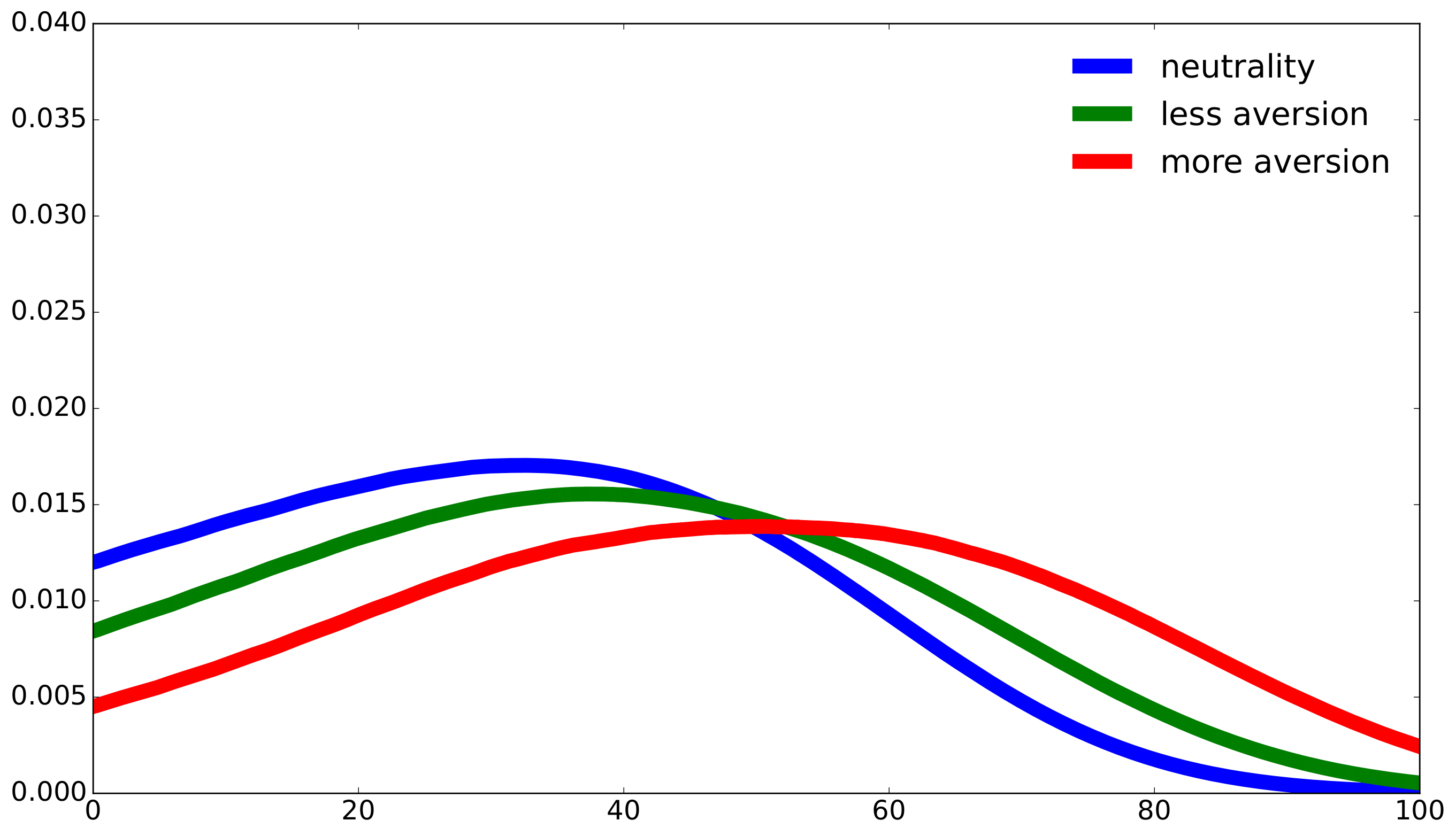
Fig. 10.1 Density for the time of the technology jump.