
6. Likelihood Ratio and Score Processes#
Authors: Lars Peter Hansen (University of Chicago) and Thomas J. Sargent (NYU)
\(\newcommand{\eqdef}{\stackrel{\text{def}}{=}}\)
6.1. Introduction#
In this chapter we study the behavior of likelihood ratio processes and score processes. We treat these as processes so that we can study their dynamic behavior when additional observations are included.
6.2. Multiplicative martingales#
Let \(\{ M_t : t \ge 0\}\) denote a process whose logarithm evolves as:
Thus the logarithmic counterpart is recognizable as an additive functional as studied in Chapter 4. We call such an \(\{ M_t : t \ge 0\}\) a multiplicative functional. We explore properties of such processes in some generality in Chapter 7. In this chapter, the processes of interest are multiplicative martingales:
Definition 6.1
The process \(M\) is a multiplicative martingale if
and thus \(E\left(M_{t+1} \mid M_t, X_t \right) = M_t.\)
Multiplicative martingales provide a convenient way to construct alternative probabilities.
Proposition 6.1
Suppose that \(\{ M_t : t \ge 0 \}\) is a multiplicative martingale. The ratio \(M_{t+1}/M_t\) implies a transition probability conditioned on \(X_t\) via the formula:
The resulting process for \(X\) remains Markovian, and the implied \(\tau\)-period transition probability can be represented as:
Proof. The linear operator:
maps nonnegative functions into nonnegative functions and the unit function into itself. Thus this operator is a conditional expectation. Moreover, it maps functions of \((w,x)\) into functions of \(x\) alone. This implies that \(\{X_t : t \ge 0\}\) is a first-order Markov process under the implied change of probability. The representation of the implied \(\tau\)-period conditional expectation operator follows from the Law of Iterated Expectations.
Remark 6.1
Under the change of measure induced by \(M_{t+1}/M_t\), the shock \(W_{t+1}\) typically does not have conditional mean zero.
So far we have not restricted the initial condition \(M_0\). We have only characterized its stochastic evolution. Suppose that the process \(\{X_t \}\) is stationary with probability denoted \(Q\), and consider \(M_0 = \tilde q(X_0)\) where \(\tilde q\) satisfies:
for all bounded (measurable) functions \(f\) of the Markov state \(x\). Then \({\widetilde Q}(dx) \eqdef {\tilde q}(x) Q(dx)\) is a stationary distribution under the implied \(\widetilde \cdot\) probability distribution.
In what follows we will impose such an initial condition on \(M_0\) so that we can apply a Law of Large Numbers as characterized in Chapter 1. In addition we will impose the ergodic restriction that the only solutions to the equation:
are constant functions with \({\tilde Q}\) measure one as investigated in Chapter 2.
6.3. Multiple models#
So far, we have considered two models, an initial one and a second one implied by a multiplicative martingale. Now suppose we have \(\ell\) such models, given an initial one and \(\ell - 1\) multiplicative martingales in addition to the initial one with multiplicative martingale equal to one. We denote each such martingale as \(\{M^i_t : t \ge 0\}\) where each one induces a process that is stationary and ergodic, with \(M^1_t = 1\) for all \(t\ge 0\). In terms of Chapter 1, think of this as partitioning sample space into \(\ell\) partitions. Each partition is matched to one of the martingales, which in turn gives the probabilities conditioned on being in that partition.
In this construction, we chose to normalize model one to be the probability distribution used for representing all of the probabilities of the martingales. Suppose instead we had used model two for this purpose. Now the \(\{M^i_t : t \ge 0\}\)’s cease to be martingales because we have changed the underlying probability from model one to model two. The ratio processes \(\{ M_t^i/M_t^2 : t \ge 0 \}\) are multiplicative martingales under this change in the underlying probability. This change in modeling perspective will be central in the discussion that follows.
6.4. Some Large Sample Properties#
We next consider two gradient inequalities that we will use prominently. The function \(m\log m\) is convex and the function \(\log m\) is concave. A convex function lies above its gradient approximation and a concave function lies below its gradient. Observe that the gradient is one for both functions when \(m=1\) and the gradient approximation is \(m-1\). Fig. 6.1 illustrates these two inequalities.
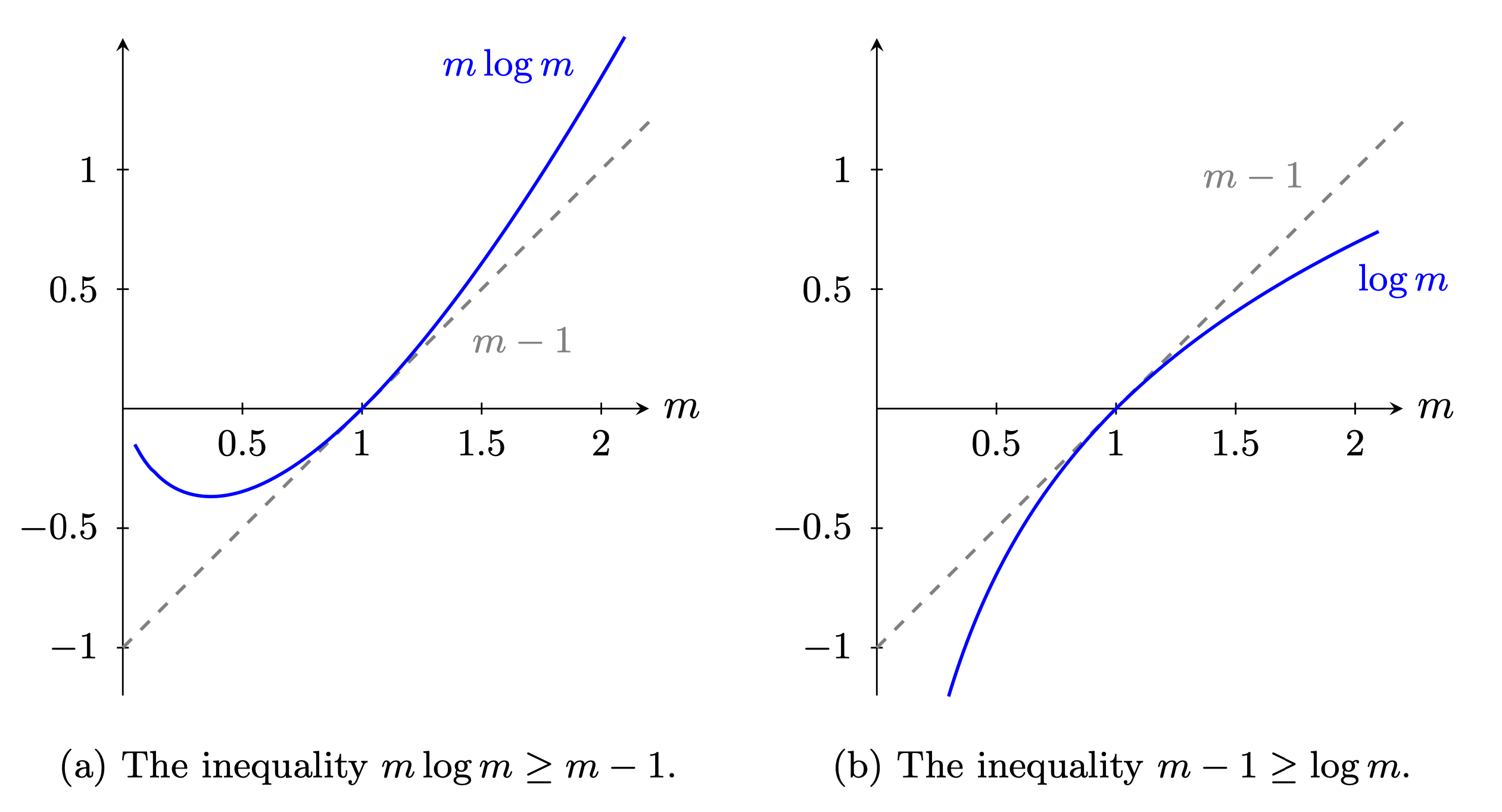
Fig. 6.1 Gradient inequalities#
We use these inequalities in conjunction with conditional expectations to obtain the targets of interest. This amounts to an application of what is called Jensen’s Inequality and implies
These weak inequalities become strict when \(\log M_{t+1} - \log M_t\) is not equal to zero with probability one. Observe that \(\{ \log M_t : t \ge 0\}\) is an additive functional of the type studied in Chapter 4 with a negative trend coefficient. A consequence of the Law of Large Numbers and the second inequality in (6.1) is that:
Suppose now we consider expectations under the probabilities implied by the multiplicative martingale \(\{M_t \ge 0\}\). Then the first inequality in (6.1) implies that
These two limits give a large sample justification for using the criterion
to determine which of the two models generates the data since the inequalities are strict when the multiplicative martingale is not degenerate. This insight extends directly to the case of multiple models captured by alternative multiplicative martingales. It leads to the use of
as a way to select models with a large sample justification. This has a direct extension to the method of maximum likelihood.
We conclude this section by pointing to unusual sample path properties of multiplicative martingales.
Theorem 6.1
For a nondegenerate multiplicative martingale, \(\{M_{t} : t \ge 0 \}\) converges almost surely to zero even though \(E\left( \frac{M_{t}}{M_0} \mid X_0 \right) = 1\) for each \(t\).
Proof. We have observed that by the Law of Large Numbers:
converges to a negative limit almost surely. This in turn implies that
almost surely.
6.5. Loglikelihoods#
We now give a particular construction of the function \(\kappa\). Let \(\theta\) denote a parameter vector and suppose that a vector of data at date \(t+1\), \(Z_{t+1}\), is given by
where \(\psi(z^* \mid x, \theta)\) is the density of \(Z_{t+1}\) given \(X_{t}\) and \(\theta\). We further assume that given \((x, \theta)\), \(Z_{t+1}\) is informationally equivalent to \(W_{t+1}\). This can be justified by assuming that we can invert \(\phi\) as a function of \(W_{t+1}\). We assume that given \(\theta\), \(X_t\) is revealed by past \(Z_t\) and possibly a finite number of lags. With this construction, we think of model \(\theta_1\) as the baseline used for computing expectations.
By factoring a joint density, we obtain a likelihood process conditioned on \((X_0, \theta)\) as:
We apply our previous arguments to justify finding the
for a discrete set of models.[1]
6.6. Score Processes#
In this section, we study first-order necessary conditions associated with the maximum likelihood estimator. For simplicity, suppose that the parameter space \(\Theta\) is an open interval of \(\mathbb{R}\) containing \(\theta_1\). Inequality (6.1) implies that the parameter value \(\theta_1\) necessarily maximizes the objective
Suppose that we can differentiate under the integral sign in (6.2) to get the first-order condition
Definition 6.2
The score process \(\{S_{t} : t = 0,1,\ldots \}\) is defined as
Theorem 6.2
\(E \left(S_{t+1} - S_t \mid X_t \right) = 0\), so the score process is an additive functional; in particular, it is a martingale with increment \(\frac{d}{d \theta} \log \psi(Z_j|X_{j-1}, \theta_1)\) under the \(\theta_1\) probability model. So
where \(V = E \left( \left[ \frac{d}{d \theta} \log \psi(Z_{t+1} |X_t, \theta_1)\right]^2 \right)\).
Proof. This follows directly from equation (6.3) and Proposition 3.2.
Theorem 6.2 justifies using the martingale central limit theorem Proposition 3.2 to characterize the large sample behavior of the score process. The resulting central limit approximation yields a large sample characterization of the maximum likelihood estimator of \(\theta\) in a Markov setting. With additional regularity conditions, the following result is typical:
where \(\theta_t\) maximizes the log likelihood function \(L_t(\theta)\). This analysis has a direct extension to the case where \(\theta\) is a vector rather than a scalar. This kind of result motivates interpreting the covariance of the martingale increment of the score process
as a measure of the information in the data about the parameter \(\theta_o\). The matrix \(V\) is called the Fisher information matrix after the statistician R.A. Fisher.
6.6.1. Nuisance Parameters#
Consider extending the notion of Fisher information to the following situation. There is a vector \(\theta\) of unknown parameters. We mainly want information about one component of the parameter vector, although to get that information we have to estimate other components too. Call the first component of \(\theta\) the ‘parameters of interest’ \(\theta_o\) and call the other component the ‘nuisance parameters’ \(\vartheta_o\). Suppose that the likelihood is parameterized on an open set \(\Theta\) in a finite dimensional Euclidean space and that the true parameter vector is \((\theta_o, \vartheta_o) \in \Theta\). Write the multivariate score process as
where \(\{ S_{t+1} : t=0,1,\ldots\}\) is the partial derivative of the log-likelihood with respect to \(\theta\) and \(\{ \tilde{S}_{t+1} : t=0,1,\ldots \}\) is the partial derivative with respect to \(\vartheta\). Estimating \(\vartheta_o\) simultaneously with \(\theta_o\) is more difficult than estimating \(\theta_o\) when \(\vartheta_o\) is known. Fisher’s measure of information corrects for the additional challenge of estimating \(\vartheta_o\) simultaneously in order to make inferences about \(\theta_o\). In particular, Fisher’s measure of information about \(\theta\) is the inverse of the \((1,1)\) component of the covariance matrix partitioned conformably with \(\theta, \vartheta\):
To represent this inverse in a useful way, compute the population regression
where \(\beta\) is the population regression coefficient and \(U_{t+1}\) is the population regression residual that by construction is orthogonal to the regressor \((\tilde{S}_{t+1} - \tilde{S}_t)\). The population regression induces the representation
which, because \(U_{t+1}\) is orthogonal to \(\tilde{S}_{t+1} - \tilde{S}_t\), implies
This equation reveals that the \((1,1)\) component of the partition of matrix \(V^{-1}\) is
The population regression equation (6.4) implies that the Fisher information measure \(E[(U_{t+1})^2]\) is no larger than \(E[(S_{t+1} - S_t)^2]\). Thus,
This inequality asserts that the likelihood function contains more information about \(\theta\) when \(\vartheta\) is known to be \(\vartheta_o\) than when \(\theta\) and \(\vartheta\) are both unknown.
Inequality (6.5) offers reasons to be cautious when interpreting calibration exercises in macroeconomics. Pretending that you know \(\vartheta\) leads you to overstate the information in the sample about the parameter \(\theta\).
Since the multivariate score \(\begin{bmatrix} S_{t+1} \\ \tilde{S}_{t+1} \end{bmatrix}\) is a vector of additive martingales, the score regression residual process \(\{ U_{t+1} : t=0,1,\ldots \}\) is itself an additive martingale.