3 Two Capital Model

This Julia notebook covers the environment in Section 4.6 with two capital stocks, which evolve as:

\[ dK_t^j = K_t^j \left[ \Phi^j \left( \frac{I_t^j}{K_t^j} \right) + \beta^j_k Z_t^1 - \eta^j \right] dt + K_t^j \sqrt{Z_t^2} {\sigma}^j_k \cdot dB_t \]

For \(j=1,2\). The output equation is now:

\[ C_t + I_t^1 + I_t^2 = \alpha K_t^a \]

where aggregate capital is a CES aggregator of the two capital stocks:

\[ K_t^a = \left[(1-\zeta) \left(K_t^1\right)^{(1 - \tau)} + \zeta \left( K_t^2\right)^{(1 - \tau)} \right]^ {\frac 1 {1 - \tau}} \]

for \(0 \le \zeta < 1\) and \(\tau \ge 0\). Agent preferences and the \(Z^1\) and \(Z^2\) processes are identical to the baseline model. The problem is very similar to the single-capital model except that we now have an additional endogenous state variable \(\widehat Y_t = \log(K_t^2/K_t^1)\).

In addition to the model inputs from Chapter 1, we also need to specify the following:

Input	Notation in paper	Description
kappa	\(\tau\)	Share parameter
zeta	\(\zeta\)	Elasticity of substitution between two types of capital
beta1	\(\beta_k^1\)	Loading factor on first capital stock in the long run risk process
beta2	\(\beta_k^2\)	Loading factor on second capital stock in the long run risk process

We have experienced convergence issues when solving the three-dimensional two-capital model directly, especially with \(\rho \neq 1\). One way to overcome this is to first run a two-dimensional version of the two-capital (abstracting from \(Z^2\)) for \(\rho=1\) and use the solution to this model as an initial guess for more complex models. Even the two-dimensional case may take several hours to run; therefore, we advise against using this Jupyter Notebook directly and instead direct users to use remote-computing resources as described on the GitHub repository.

To solve the model, we first we load the necessary libraries:

include("src/3/main_twocapitals_two_dimensions.jl")
include("src/3/utils_twocapitals_two_dimensions.jl")
using Pkg
using Optim
using Roots
using NPZ
using ArgParse

  Activating project at `/project/lhansen/macrofinance`

Next, we set the model inputs for the two-dimensional model with \(\rho=1\).

Delta = 1.0
gamma = 8.0
rho = 1.0
alpha = 0.1844
kappa = 0.0
zeta = 0.5
beta1 = 0.01
beta2 = 0.01
action_name = "test"

"test"

Now we can run main_2d with the above inputs:

main_2d(Delta, gamma, rho, alpha, kappa, zeta, beta1, beta2, action_name)

This gives us a solution for \(\rho=1\). If we are interested in \(\rho \neq 1\), we use this first solution as an initial guess for the other values of \(\rho\). For example, to solve for \(\rho=0.67\):

rho = 0.67
main_2d(Delta, gamma, rho, alpha, kappa, zeta, beta1, beta2, action_name)

Next, we can use these solutions as initial guesses for their three-dimensional counterparts. For example, for the \(\rho=1\) counterpart:

include("src/3/main_twocapitals_three_dimensions.jl")
include("src/3/utils_twocapitals_three_dimensions.jl")
rho = 1.0
main_3d(Delta, gamma, rho, alpha, kappa, zeta, beta1, beta2, action_name)

The outputs of the solution are the same as for the baseline model except for the additional state variables for \(\hat{Y}_t\), such as smean for \(\mu_{\hat{y}}\) and sigma_s.

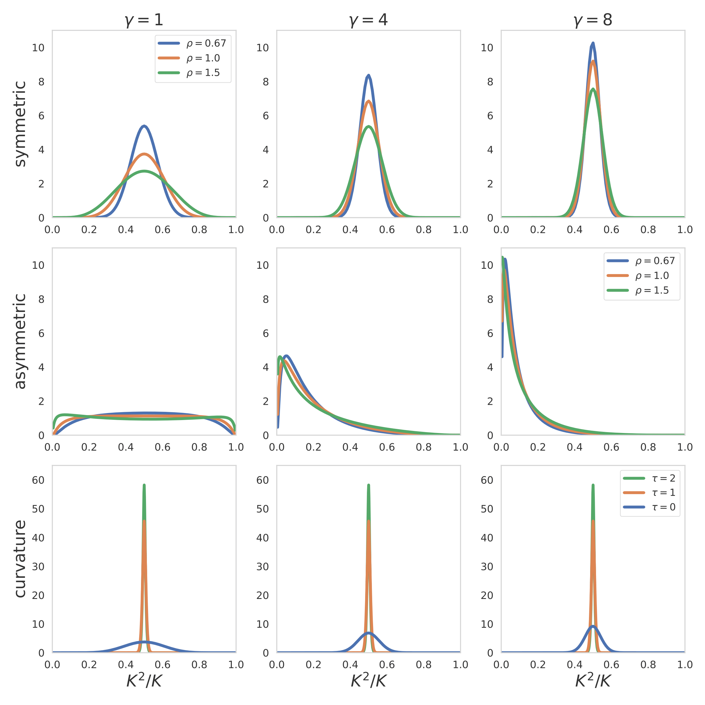
Fig. 1 Example taken from Figure 7 of the paper.