4 Heterogeneous Agents

4 Heterogeneous Agents#

This Python notebook covers the environment in section 5. We need to solve the following:

Expert’s HJB equation

\[\begin{align*} \begin{split} {L}^e_{HJB} \left(v^e, v^h, \kappa, \chi;x \right) &= \frac{\rho_e}{1-\rho_e} \delta_e^{1 / \rho_e} \exp\left[({1- \frac{1}{\rho_e}})v^e)\right]-\frac{\delta_e}{1-\rho_e}+r\\&+\frac{1}{2 \gamma_e} \frac{\left(\Delta^e+\pi^h \cdot \sigma_R\right)^2}{\left\|\sigma_R\right\|^2} +\left[\mu_X+\frac{1-\gamma_e}{\gamma_e}\left(\frac{\Delta^e+\pi^h \cdot \sigma_R}{\left\|\sigma_R\right\|^2}\right) \sigma_X \sigma_R\right] \cdot \partial_X v^e \\ &+\frac{1}{2}\left[\operatorname{tr}\left(\sigma_X^{\prime} \partial_{xx^{\prime}} v^e \sigma_X\right)+\frac{1-\gamma_e}{\gamma_e}\left(\sigma_X^{\prime} \partial_x v_e\right)^{\prime}\left[\gamma_e \mathbb{I}_d+\left(1-\gamma_e\right) \frac{\sigma_R \sigma_R^{\prime}}{\left\|\sigma_R\right\|^2}\right] \sigma_X^{\prime} \partial_x v^e\right]= 0 \end{split} \end{align*}\]

Household’s HJB equation

\[\begin{align*} \begin{split} {L}^h_{HJB} \left(v^e, v^h, \kappa, \chi;x \right) &= \frac{\rho_h}{1-\rho_h} \delta_h^{1 / \rho_h} \exp\left[\left(1- \frac{1}{\rho_h}\right)v^h\right] - \frac{\delta_h}{1-\rho_h} + r \\ &+ \frac{1}{2 \gamma_h}\|\pi^h\|^2 \\ &+ \left[\mu_X + \frac{1-\gamma_h}{\gamma_h} \sigma_X \pi^h\right] \cdot \partial_x v^h \\ &+ \frac{1}{2}\left[\operatorname{tr}\left(\sigma_X^{\prime} \partial_{xx^{\prime}} v^h \sigma_X\right) + \frac{1-\gamma_h}{\gamma_h}\left\|\sigma_X^{\prime} \partial_x v^h\right\|^2\right] = 0 \end{split} \end{align*}\]

Optimal expert capital share

\[\begin{align*} \begin{split} {L}_{\kappa} \left(v^e, v^h,\kappa, \chi;x \right) &= \min\Big\{ 1 - \kappa, \, w\gamma_h (1-\chi\kappa) | \sigma_R |^2 - (1-w) \gamma_e \chi \kappa | \sigma_R |^2 \\ &+ w(1-w) \frac{\alpha_e - \alpha_h}{\underline{\chi} q} \\ &+ w(1-w) \left( \sigma_x \sigma_R \right) \cdot \left[ (\gamma_h-1)\partial_x \upsilon^h - (\gamma_e-1)\partial_x \upsilon^e \right] \Big\} = 0 \end{split} \end{align*}\]

Optimal expert equity retention

\[\begin{align*} \begin{split} {L}_{\chi} \left(v^e, v^h, \kappa, \chi;x \right) &= \min\Big\{ \chi - \underline{\chi}, \, \Big[ ((1-w)\gamma_e + w\gamma_h) | D_{z} |^2 + (\partial_w \log q) D_{\upsilon,z} - D_{\upsilon,w} \Big](\chi - w) \\ &+ w(1-w) (\gamma_e - \gamma_h) | D_{z} |^2 - D_{\upsilon,z} \Big\} = 0 \end{split} \end{align*}\]

Where:

\[\begin{align*} D_{z} &\doteq \sqrt{z_2}\sigma_k + \sigma_{z}' \partial_{z} \log q \\ D_{\upsilon,w} &\doteq w(1-w) | D_{z} |^2 \partial_w \big[ (\gamma_h - 1) \upsilon^h - (\gamma_e - 1)\upsilon^e \big] \\ D_{\upsilon,z} &\doteq w(1-w) \left(\sigma_{z}D_{z} \right) \cdot \partial_{z} \big[ (\gamma_h - 1) \upsilon^h - (\gamma_e - 1)\upsilon^e \big] \end{align*}\]

Since $\chi$ can be solved algebraically, we solve (1) to (3).

4.1 Solution Overview#

4.1.1 Model Architecture#

We modify the DeepGalerkinMethod code from the companion code to Correia et. al 2018. We construct a feedforward, fully-connected neural network to approximate $v^e$, $v^h$ and $\kappa$ as functions of the states.

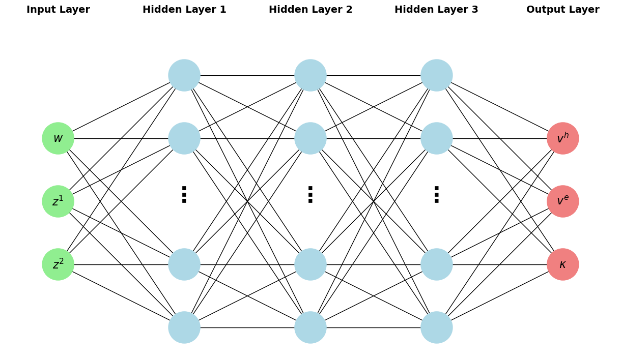
_images/neural_network.png — Fig. 2 Neural network architecture used in this computation. Note that in the paper, `layer_width`=16.#

We employ the following hyperparameters:

Input	Description	Parameter used in paper
`n_layers`	Number of layers	2
`units`	Number of neurons in each layer	16
`input_dim`	Dimension of input into first layer	3 (This should be the same as the number of states)
`activation`	Activation function for all layers except the last	tanh
`final_activation`	Activation function for final layer	Identity function for first two dimensions; sigmoid for third dimension. This is so that…
`seed`	Seed for weight and bias initialization	256

We use a Glorot normal initializer to initialize weights and a Glorot uniform initializer to initialize the biases.

4.1.2 Training#

The training set is constructed by drawing uniformly from the three-dimensional cube bounded by [wMin,zMin,vMin] and [wMax,zMax,vMax]. The loss function is given by the mean squared error of $L$, where:

\[ L = {L}^e_{HJB} + {L}^h_{HJB} + p{L}_{\kappa} \]

Where $p$ is a penalization parameter. We compute gradients using tf.GradientTape and use an L-BFGS-B solver. For the settings used in the paper, there are 659 trainable variables: 3x16 weights and 16 bias terms for the initial layer; 16x16 weights and 16 bias terms for each hidden layer; and 16x3 weights and 3 bias terms for the final layer. The full list of parameters for the training stage are:

Input	Description	Parameter used in paper
`points_size`	Determines the `batchSize`, which is $2^x$ where $x$ is `points_size`. Batch size is the number of training samples in each epoch	10
`iter_num`	Number of epochs, i.e. the number of complete passes through the training set	5
`penalization`	Penalty for violating $\kappa$ constraint	10000
`seed`	Seed for drawing uniform samples	256 (same as seed for initialization)
`max_iter`	Maximum number of L-BFGS-B iterations (number of times parameters are updated) per epoch	100
`maxfun`	Maximum number of function evaluations per epoch	100
`maxcor`	The maximum number of variable metric corrections used to define the limited memory matrix used to compute the Hessian per epoch	100
`maxls`	Maximum number of line search steps per iteration used to find the optimal step-size	100
`gtol`	Iteration will stop when $\max\|proj(g_i)\| \leq$ `gtol` for each entry $i$ of the (projected) gradient vector	Machine epsilon for float64 (~$2^{-16}$)
`ftol`	Iteration will stop when $\frac{L^k - L^{k+1}}{\max{\|L^k\|,\|L^{k+1}\|,1}} \leq$ `ftol`	Machine epsilon for float64 (~$2^{-16}$)
`tolerance`	Iteration will stop when, after fully completing an epoch, $L$ is less than `tolerance`	$10^{-5}$

4.1.3 Model Parameters#

We also need to set model parameters. These will vary depending on the environment chosen from Section 5.1. By default, the following parameters are allowed as inputs to main_BFGS:

Input	Description	Parameter used in paper
`chiUnderline`	Skin-in-the-game constraint	$\underline{\chi}$
`gamma_e`, `gamma_h`	Expert and household uncertainty aversion	$\gamma_e, \gamma_h$
`a_e`, `a_h`	Expert and household productivity	$\alpha_e, \alpha_h$
`delta_e`,`delta_h`	Expert and household discount rate	$\delta_e, \delta_h$
`rho_e`,`rho_h`	Expert and household inverse of IES	$\rho_e, \rho_h$
`lambda_d`	Birth/death rate	$\lambda_d$
`nu`	Fraction of newborns which are experts	$\nu$
`V_bar`	Mean of $Z_2$	$\mu_2$
`sigma_K_norm`, `sigma_Z_norm`, `sigma_V_norm`	Normalization for variances; these are multiplied by the covariance matrix specified in `utils_para` to yield $\sigma_k, \sigma_1, \sigma_2$
`wMin`, `wMax`	Bounds for training set for $W$; the corresponding bounds for $Z_1$ and $Z_2$ can be edited in `utils_para`
`nWealth`, `nZ`, `nV`	Number of gridpoints for each state variable; this does not have any effect on the solution but will determine the evaluation of variables of interest using the solution at a later step
`shock_expo`	Determines whether the shock exposure matrix is “upper_triangular” or “lower_triangular”

In addition, the following parameters can be edited in the utils_para file. They do not vary across the models explored in the paper, but the user may wish to explore their own variations.

Input	Description	Notation used in paper	Default used in paper
`Z_bar`	Mean of $Z^1$		0.0
`lambda_Z`	Persistence of $Z^1	$\beta_1$	0.056
`lambda_V`	Persistence of $Z^2$	$\beta_2$	0.194
`alpha_K`	$\eta_k$	$\alpha$	0.04
`phi`	Adjustment cost	$\phi$	8.0
`covij`	$i,j$ entry in shock exposure matrix		See Table 1 in paper
`numSds`	Governs grid size for $Z^1$ and $Z^2$ (number of standard deviations from the mean)		5
`zmin`,`zmax`	Grid boundaries for $Z^1$		$\mu_1 \pm SD\cdot Var(Z_1\|Z_2=\mu_2)$ where $SD=$`numSds`
`vmin`,`vmax`	Grid boundaries for $Z^2$		`vmin` = $10^{-8}$,`vmax` = $\mu_2 + SD\cdot Var(Z_2\|Z_2=\mu_2)$ where $SD=$`numSds`

4.2 Quick Start#

We can build and train the neural network as follows. First, we import libraries:

import json
import numpy as np
import tensorflow as tf 
import time 
import os
os.chdir("src/4")
from main_BFGS import main
from utils_para import setModelParameters
from utils_training import training_step_BFGS
from utils_DGM import DGMNet
os.chdir("../..")
import warnings
warnings.filterwarnings("ignore")
tf.get_logger().setLevel('ERROR')
tf.config.set_visible_devices([], 'GPU')

Next, we set the model parameters and hyperparameters. In the following example, we have used a variant of Model RF.

chiUnderline = 1.0
gamma_e = 4.0
a_e=0.0922
a_h=0.0
gamma_h=4.0
delta_e=0.0115
delta_h=0.01
lambda_d=0.0
rho_e=1.0
rho_h=1.0
nu=0.1

V_bar=0.0000063030303030303026
sigma_K_norm=3.1707442821755683
sigma_Z_norm=19.835431735873996
sigma_V_norm=0.0010882177801089308
wMin=0.01
wMax=0.99

nWealth=180
nZ=30
nV=30

seed_=(256)
n_layers_=(2)
units_=(16)
points_size_=(10)
iter_num_=(5)
penalization=10000

BFGSmaxiter=100
BFGSmaxfun=100
action_name = 'test'

seed=256
n_layers=2
units=16
points_size=10
iter_num=5
penalization=10000
BFGS_maxiter=100
BFGS_maxfun=100
shock_expo = 'upper_triangular'

Next, we run the main solution, which trains the neural network. Under the parameterization above, this will take around 1 minute.

main(action_name, nWealth, nZ, nV, V_bar, sigma_K_norm, sigma_Z_norm, sigma_V_norm, wMin, wMax, chiUnderline, a_e, a_h, gamma_e, gamma_h, rho_e, rho_h, delta_e, delta_h, lambda_d, nu, shock_expo, n_layers, points_size, iter_num, units, seed, penalization, BFGS_maxiter, BFGS_maxfun)

Now that we have a solution, we can compute variables of interest, which can subsequently be used to compute shock elasticities. By default, main_variable computes the following variables. Unless specified otherwise, the variables are evaluated on an array with dimension [nWealth,nZ,nV].

Output	Description	Notation used in paper
`W_NN`, `Z_NN`, `V_NN`	The values of $W$, $Z_1$ and $Z_2$ on the state-space grid
`XiE_NN`, `XiH_NN`	Expert and household value functions	$V_e$, $V_h$
`logXiE_NN`, `logXiH_NN`	Log expert and household value functions	$\hat{V}_e$, $\hat{V}_h$
`chi_NN`	Expert equity retention	$\chi$
`kappa_NN`	Expert capital share	$\kappa$
`r_NN`	Risk-free rate	$r$
`q_NN`	Price of capital	$Q$
`sigmaW_NN`,`sigmaZ_NN`,`sigmaV_NN`	State volatilities	$Z^2 \sigma_w$,$Z^2 \sigma_1$, $Z^2 \sigma_2$
`muW_NN`,`muZ_NN`,`muV_NN`	State drifts	$\mu_w$,$\mu_1$,$\mu_2$
`muK_NN`	Log capital drift	$\mu_{k}$
`sigmaK_NN`	Log capital diffusin	$\sigma_{k}$
`muQ_NN`	Capital price drift	$\mu_q$
`sigmaQ_NN`	Capital price diffusion	$\sigma_q$
`sigmaR_NN`	Capital return volatility	$\sigma_r$
`deltaE_NN`, `deltaH_NN`	Expert and household risk premium wedge	$\Delta^e$,$\Delta^h$
`PiE_NN`, `PiH_NN`	Expert and household equity risk price	$\pi_e$,$\pi_h$
`betaE_NN`,`betaH_NN`		$\frac{\chi \kappa}{W}$, $\frac{1- \kappa}{W}$
`HJB_E_NN`, `HJB_H_NN`, `kappa_min_NN`	RHS of HJB equations and $\kappa$ constraint evaluated on the state space grid	$L^e$, $L^h$, $L^{\kappa}$
`HJBE_validation_MSE`, `HJBH_validation_MSE`, `kappa_validation_MSE`	Loss function (scalar)
`dent_NN`	Stationary density
`dX_logXiE_NN`, `dX_logXiH_NN`, `dX2_logXiE_NN`, `dX2_logXiH_NN`	First and second derivatives of expert and household value function with respect to each of the states; separate objects for each state are also included
`mulogSe_NN`, `mulogSh_NN`	Log SDF drifts for expert and household	$-r_t S_t^e$, $-r_t S_t^h$
`sigmalogSe_NN`, `sigmalogSh_NN`	Log SDF diffusions for expert and household	$-S_t^e \pi_t^e$, $-S_t^h \pi_t^h$
`mulogCe_NN`, `mulogCh_NN`	Log consumption drifts for expert and household	$\hat{\mu}_c^e$, $\hat{\mu}_c^h$
`sigmalogCe_NN`, `sigmalogCh_NN`	Log consumption diffusions for expert and household	$\sigma_c^e$, $\sigma_c^h$
`mulogC_NN`	Log aggregate consumption drift	$\hat{\mu}_c$
`sigmalogC_NN`	Log aggregate consumption diffusion	$\sigma_c$

Given that a solution has been saved under the same parameters, the following code outputs the variables listed above. In addition, the marginal_quantile_func_factory function is called to save the above outputs evaluated at desired quantiles (e.g. $Z^2$ at median) for ease of plotting.

os.chdir('src/4')
from main_variable import main_var
os.chdir('../..')

main_var(action_name, nWealth, nZ, nV, V_bar, sigma_K_norm, sigma_Z_norm, sigma_V_norm, wMin, wMax, chiUnderline, a_e, a_h, gamma_e, gamma_h, rho_e, rho_h, delta_e, delta_h, lambda_d, nu, shock_expo, n_layers, units, points_size, iter_num, seed, penalization, BFGS_maxiter, BFGS_maxfun)

2024-09-03 01:55:37.533890: I tensorflow/core/platform/cpu_feature_guard.cc:193] This TensorFlow binary is optimized with oneAPI Deep Neural Network Library (oneDNN) to use the following CPU instructions in performance-critical operations:  AVX2 AVX512F AVX512_VNNI FMA
To enable them in other operations, rebuild TensorFlow with the appropriate compiler flags.

4.3 Plotting#

We can now plot the results.

import os
import numpy as np
os.chdir('src/4')
from plot import return_NN_solution
os.chdir('../..')
import matplotlib.pyplot as plt
import seaborn as sns
sns.set(style="whitegrid", font_scale=1.13, rc={"lines.linewidth": 3.5})
plt.rcParams['axes.formatter.useoffset'] = True

First we load in the results using the same parameters as before.

results = return_NN_solution(shock_expo=shock_expo, seed=seed, chiUnderline=chiUnderline, a_e=a_e, a_h=a_h, gamma_e=gamma_e, gamma_h=gamma_h, psi_e=rho_e, psi_h=rho_h, delta_e=delta_e, delta_h=delta_h, lambda_d=lambda_d, nu=nu, n_layers=n_layers, units=units, iter_num=iter_num, points_size=points_size, penalization=penalization, action_name=action_name)

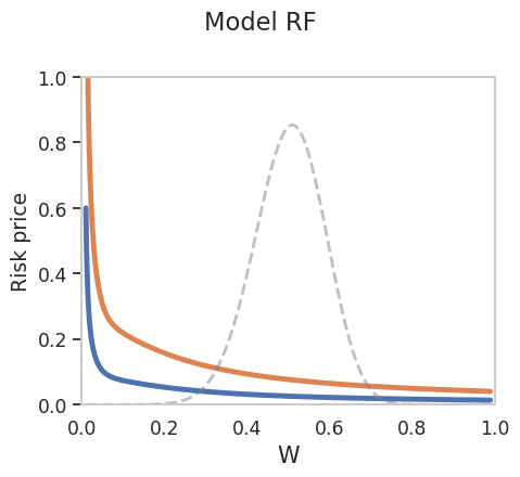
We provide an example plot below. Notice that we use results['eva_V_10'] and results['eva_V_90'] to extract the variables of interest evaluated at $Z^1=0$ and $Z^2$ at its 10th and 90th percentiles, respectively.

fig, ax = plt.subplots(1,1, figsize=(5,4.5))
W_dense = np.unique(results['eva_V_50']['W'])
W_sparse = np.unique(results['W'].values)
sns.lineplot(x = W_dense, y = results['eva_V_10']['PiE_NN'][:,0], ax = ax)
sns.lineplot(x = W_dense, y = results['eva_V_90']['PiE_NN'][:,0], ax = ax)
ax2 = ax.twinx()
sns.lineplot(x = W_sparse, y = results['dentW'].values, ax = ax2, ls='--', color='grey',lw=2.0, alpha=0.5)
ax2.grid(False)
ax2.set_yticks([])
ax2.set_ylim([0,0.03])

ax.set_xlim(0,1.0)
ax.grid(False)
ax.set_ylim([0.0,1.0])
ax.set_xlabel('W', fontsize=15)
ax.set_ylabel('Risk price')
plt.suptitle("Model RF")

plt.tight_layout()

_images/f58b3fd9d9a5e0ed1b75bbd2cad94788e77c19aa1767b22340bdd78602925c30.png

4.4 Finite Difference Method#

We employ a finite differences method from mfrSuite to solve the two-dimensional Model IP from Section 5, which we cover briefly here.

import mfr.modelSoln as m
import numpy as np
import argparse
import os
import sys
import warnings
warnings.filterwarnings("ignore")
os.chdir('src/5')
from main_solve import main_fdm
from main_evaluate import interpolate
os.chdir('../..')

The model inputs are identical to the neural network solution above, except that: we abstract away from $Z^2$; we have to set $dt$, the false-transient time-step; and some inputs have been moved inside the main_solve.py script.

chiUnderline = 1.0
a_e=0.0922
a_h=0.085
gamma_e = 2.0
gamma_h= 2.0
delta_e=0.03
delta_h=0.01
lambda_d=0.0
rho_e=1.0
rho_h=1.0
nu=0.1
dt = 0.1
nWealth=180
nZ=30
shock_expo = 'upper_triangular'
action_name = 'test'

main_fdm(nW=nWealth, nZ=nZ, dt=dt, a_e=a_e, a_h=a_h, rho_e=rho_e, rho_h=rho_h, gamma_e=gamma_e, gamma_h=gamma_h, chiUnderline=chiUnderline, action_name=action_name, shock_expo=shock_expo, delta_e=delta_e, delta_h=delta_h, lambda_d=lambda_d, nu=nu)

Show code cell output Hide code cell output

Program converged. Took 8089 iterations and 199.59 seconds. 2.49% of the time was spent on dealing with the linear systems.
Parameter            Value     
nu_newborn           0.1       
lambda_d             0.0       
lambda_Z             0.056     
lambda_V             0.0       
lambda_Vtilde        0.0       
Z_bar                0.0       
V_bar                1.0       
Vtilde_bar           0.0       
sigma_K_norm         0.008696916904073742
sigma_Z_norm         0.049798518005773194
sigma_V_norm         0.0       
sigma_Vtilde_norm    0.0       
nWealth              180       
nZ                   30        
nV                   0         
nVtilde              0         
nDims                2         
delta_e              0.03      
delta_h              0.01      
a_e                  0.0922    
a_h                  0.085     
rho_e                1.0       
rho_h                1.0       
phi                  8.0       
gamma_e              2.0       
gamma_h              2.0       
equityIss            2         
hhCap                1         
chiUnderline         1.0       
method               2         
dt                   0.1       
dtInner              0.1       
tol                  1e-05     
innerTol             1e-05     
maxIters             500000    
maxItersInner        500000    
iparm_2              28        
iparm_3              0         
iparm_28             0         
iparm_31             0         
numSds               5         
wMin                 0.001     
wMax                 0.999     
logW                 -1        
folderName           output/test/upper_triangular/dt_0.1/nW_180_nZ_30/chiUnderline_1.000/a_e_0.092_a_h_0.085/gamma_e_2.000_gamma_h_2.000/rho_e_1.000_rho_h_1.000/delta_e_0.030_delta_h_0.010/lambda_d_0.000_nu_0.100
overwrite            Yes       
verbatim             -1        
exportFreq           1000000   
cov11                0.9153150324227657
cov12                0.4027386142660167
cov21                0.0       
cov22                1.0       
Exporting solution information: time used, convergence error, etc.
Exporting state variables.
==========================================
Exporting numerical results.
==========================================
(1): Exporting risk prices and interest rate: q, piH, piE, deltaE, deltaH, r, I.
------------------------------------------------
(2) Exporting drifts: muQ, muX, muK, muRe, muRh.
------------------------------------------------
(3) Exporting vols: sigmaQ, sigmaR, sigmaK.
------------------------------------------------
(4) Exporting value and policy functions: XiE, XiH, cHatE, cHatH, kappa, chi, betaE, betaH.
------------------------------------------------
(5) Exporting derivs: first, second, and cross derivs of XiE and XiH.
------------------------------------------------
(6) Exporting the rest: experts' leverage, sigmaC, sigmaCe, sigmaCh, sigmaSe, sigmaSh, simgaLogY, muC, muCe, muCh, muY, muSe, muSh.
------------------------------------------------
Exporting matrices' information
==========================================
(1) Exporting matrix coefficients
------------------------------------------------
(2) Exporting matrices and RHSs.
------------------------------------------------

Before we can plot any variables of interest, we need to interpolate on our state space grid. Here we interpolate risk prices linearly using scipy.interpolate.griddata.

interpolate(nW=nWealth, nZ=nZ, dt=dt, a_e=a_e, a_h=a_h, rho_e=rho_e, rho_h=rho_h, gamma_e=gamma_e, gamma_h=gamma_h, chiUnderline=chiUnderline, action_name=action_name, shock_expo=shock_expo, delta_e=delta_e, delta_h=delta_h, lambda_d=lambda_d, nu=nu)

Now we can load and plot our results:

import pandas as pd
import pickle
np.set_printoptions(suppress=True, linewidth=200)
import matplotlib.pyplot as plt
import seaborn as sns
sns.set(style="whitegrid", font_scale=1.13, rc={"lines.linewidth": 3.5})
plt.rcParams['axes.formatter.useoffset'] = True
os.chdir("src/5")
from plot import return_fdm_solution
os.chdir("../..")
fdm_result = return_fdm_solution(shock_expo=shock_expo, dt=dt, nW=nWealth, chiUnderline=chiUnderline, a_e=a_e, a_h=a_h, gamma_e=gamma_e, gamma_h=gamma_h, rho_e=rho_e, rho_h=rho_h, delta_e=delta_e, delta_h=delta_h, lambda_d=lambda_d, nu=nu, action_name=action_name, nZ=nZ)

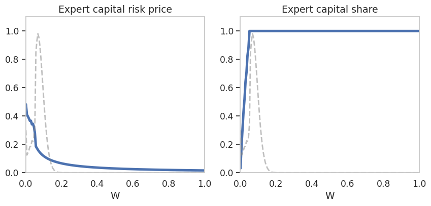
Here we plot the expert capital risk price and capital share as they vary with $W$.

fig, axes = plt.subplots(1,2, figsize=(10,4))
W = fdm_result['W']['W'].unique()

sns.lineplot(x = W, y = fdm_result['PiE_final_capital'], ax = axes[0])
ax2 = axes[0].twinx()
sns.lineplot(x = W, y = fdm_result['dents'].values, ax = ax2, ls='--', color='grey',lw=2.0, alpha=0.5)
ax2.grid(False)
ax2.set_yticks([])
ax2.set_yticklabels([])
axes[0].set_ylim(0,1.1)
axes[0].set_xlim(0,1.0)
ax2.set_ylim([0,0.1])
axes[0].title.set_text("Expert capital risk price")
axes[0].set_xlabel('W')


sns.lineplot(x = W, y = fdm_result['kappa_final'], ax = axes[1])
ax2 = axes[1].twinx()
sns.lineplot(x = W, y = fdm_result['dents'].values, ax = ax2, ls='--', color='grey',lw=2.0, alpha=0.5)
ax2.grid(False)
ax2.set_yticks([])
ax2.set_yticklabels([])
axes[1].set_ylim(0,1.1)
axes[1].set_xlim(0,1.0)
ax2.set_ylim([0,0.1])
axes[1].title.set_text("Expert capital share")
axes[1].set_xlabel('W')
axes[0].grid(False)
axes[1].grid(False)

_images/7064e3b3e9bd67f19ce7dad9e2ada481ecf808af4fdb3939d9c992481f528898.png

Input	Description	Parameter used in paper
`points_size`	Determines the `batchSize`, which is \(2^x\) where \(x\) is `points_size`. Batch size is the number of training samples in each epoch	10
`iter_num`	Number of epochs, i.e. the number of complete passes through the training set	5
`penalization`	Penalty for violating \(\kappa\) constraint	10000
`seed`	Seed for drawing uniform samples	256 (same as seed for initialization)
`max_iter`	Maximum number of L-BFGS-B iterations (number of times parameters are updated) per epoch	100
`maxfun`	Maximum number of function evaluations per epoch	100
`maxcor`	The maximum number of variable metric corrections used to define the limited memory matrix used to compute the Hessian per epoch	100
`maxls`	Maximum number of line search steps per iteration used to find the optimal step-size	100
`gtol`	Iteration will stop when \(\max\|proj(g_i)\| \leq\) `gtol` for each entry \(i\) of the (projected) gradient vector	Machine epsilon for float64 (~\(2^{-16}\))
`ftol`	Iteration will stop when \(\frac{L^k - L^{k+1}}{\max{\|L^k\|,\|L^{k+1}\|,1}} \leq\) `ftol`	Machine epsilon for float64 (~\(2^{-16}\))
`tolerance`	Iteration will stop when, after fully completing an epoch, \(L\) is less than `tolerance`	\(10^{-5}\)

Input	Description	Parameter used in paper
`chiUnderline`	Skin-in-the-game constraint	\(\underline{\chi}\)
`gamma_e`, `gamma_h`	Expert and household uncertainty aversion	\(\gamma_e, \gamma_h\)
`a_e`, `a_h`	Expert and household productivity	\(\alpha_e, \alpha_h\)
`delta_e`,`delta_h`	Expert and household discount rate	\(\delta_e, \delta_h\)
`rho_e`,`rho_h`	Expert and household inverse of IES	\(\rho_e, \rho_h\)
`lambda_d`	Birth/death rate	\(\lambda_d\)
`nu`	Fraction of newborns which are experts	\(\nu\)
`V_bar`	Mean of \(Z_2\)	\(\mu_2\)
`sigma_K_norm`, `sigma_Z_norm`, `sigma_V_norm`	Normalization for variances; these are multiplied by the covariance matrix specified in `utils_para` to yield \(\sigma_k, \sigma_1, \sigma_2\)
`wMin`, `wMax`	Bounds for training set for \(W\); the corresponding bounds for \(Z_1\) and \(Z_2\) can be edited in `utils_para`
`nWealth`, `nZ`, `nV`	Number of gridpoints for each state variable; this does not have any effect on the solution but will determine the evaluation of variables of interest using the solution at a later step
`shock_expo`	Determines whether the shock exposure matrix is “upper_triangular” or “lower_triangular”

Input	Description	Notation used in paper	Default used in paper
`Z_bar`	Mean of \(Z^1\)		0.0
`lambda_Z`	Persistence of $Z^1	\(\beta_1\)	0.056
`lambda_V`	Persistence of \(Z^2\)	\(\beta_2\)	0.194
`alpha_K`	\(\eta_k\)	\(\alpha\)	0.04
`phi`	Adjustment cost	\(\phi\)	8.0
`covij`	\(i,j\) entry in shock exposure matrix		See Table 1 in paper
`numSds`	Governs grid size for \(Z^1\) and \(Z^2\) (number of standard deviations from the mean)		5
`zmin`,`zmax`	Grid boundaries for \(Z^1\)		\(\mu_1 \pm SD\cdot Var(Z_1\|Z_2=\mu_2)\) where \(SD=\)`numSds`
`vmin`,`vmax`	Grid boundaries for \(Z^2\)		`vmin` = \(10^{-8}\),`vmax` = \(\mu_2 + SD\cdot Var(Z_2\|Z_2=\mu_2)\) where \(SD=\)`numSds`

Output	Description	Notation used in paper
`W_NN`, `Z_NN`, `V_NN`	The values of \(W\), \(Z_1\) and \(Z_2\) on the state-space grid
`XiE_NN`, `XiH_NN`	Expert and household value functions	\(V_e\), \(V_h\)
`logXiE_NN`, `logXiH_NN`	Log expert and household value functions	\(\hat{V}_e\), \(\hat{V}_h\)
`chi_NN`	Expert equity retention	\(\chi\)
`kappa_NN`	Expert capital share	\(\kappa\)
`r_NN`	Risk-free rate	\(r\)
`q_NN`	Price of capital	\(Q\)
`sigmaW_NN`,`sigmaZ_NN`,`sigmaV_NN`	State volatilities	\(Z^2 \sigma_w\),\(Z^2 \sigma_1\), \(Z^2 \sigma_2\)
`muW_NN`,`muZ_NN`,`muV_NN`	State drifts	\(\mu_w\),\(\mu_1\),\(\mu_2\)
`muK_NN`	Log capital drift	\(\mu_{k}\)
`sigmaK_NN`	Log capital diffusin	\(\sigma_{k}\)
`muQ_NN`	Capital price drift	\(\mu_q\)
`sigmaQ_NN`	Capital price diffusion	\(\sigma_q\)
`sigmaR_NN`	Capital return volatility	\(\sigma_r\)
`deltaE_NN`, `deltaH_NN`	Expert and household risk premium wedge	\(\Delta^e\),\(\Delta^h\)
`PiE_NN`, `PiH_NN`	Expert and household equity risk price	\(\pi_e\),\(\pi_h\)
`betaE_NN`,`betaH_NN`		\(\frac{\chi \kappa}{W}\), \(\frac{1- \kappa}{W}\)
`HJB_E_NN`, `HJB_H_NN`, `kappa_min_NN`	RHS of HJB equations and \(\kappa\) constraint evaluated on the state space grid	\(L^e\), \(L^h\), \(L^{\kappa}\)
`HJBE_validation_MSE`, `HJBH_validation_MSE`, `kappa_validation_MSE`	Loss function (scalar)
`dent_NN`	Stationary density
`dX_logXiE_NN`, `dX_logXiH_NN`, `dX2_logXiE_NN`, `dX2_logXiH_NN`	First and second derivatives of expert and household value function with respect to each of the states; separate objects for each state are also included
`mulogSe_NN`, `mulogSh_NN`	Log SDF drifts for expert and household	\(-r_t S_t^e\), \(-r_t S_t^h\)
`sigmalogSe_NN`, `sigmalogSh_NN`	Log SDF diffusions for expert and household	\(-S_t^e \pi_t^e\), \(-S_t^h \pi_t^h\)
`mulogCe_NN`, `mulogCh_NN`	Log consumption drifts for expert and household	\(\hat{\mu}_c^e\), \(\hat{\mu}_c^h\)
`sigmalogCe_NN`, `sigmalogCh_NN`	Log consumption diffusions for expert and household	\(\sigma_c^e\), \(\sigma_c^h\)
`mulogC_NN`	Log aggregate consumption drift	\(\hat{\mu}_c\)
`sigmalogC_NN`	Log aggregate consumption diffusion	\(\sigma_c\)