
4. Solution with price stochasticity#
We then consider model with price stochasticity. To account for stochastic prices in a tractable way, we construct an approximate Markov chain with two states \(P^a_\ell < P^a_h\) and transitions that match the empirical transitions from monthly data. We implement ``Modified Predictive Control’’ (MPC) methods for solving our planner’s problem.
4.1. Model setup#
Our MPC approximation is implemented as follows: Starting from the current period, denoted as date zero, we break the future into two segments: a) an uncertainty horizon of, say, \(h\) time periods and b) the remaining \(T- h\) time periods beyond this uncertainty horizon for which we abstract from uncertainty. Although the cattle price distribution follows a Markov chain, to simplify our computations, we set the prices in periods \(h+1, \dots T\) equal to the value that prevails at \(h.\) Prior to date \(h +1,\) we confront randomness in this problem by imposing appropriate ``measurability’’ restrictions on the controls as functions of potentially realized states.
We then apply the interior point method to find the optimal trajectory at date zero given \(P^a_0.\) We keep the optimal date \(t=1\) states computed at time \(t=0\) and repeat. That is, we consider the problem starting at \(t=1\) with the new state vector and divide the future into two segments: an uncertainty segment of length \(h\) and a remaining period of \(T-h - 1.\) This step will determine an optimal state at period 2. We continue this procedure to produce the optimal state at periods 3, 4, …, T supported by the corresponding optimal controls.
Mathematically, label the potential state realizations as \(j=1,2,...,n\). Let \(\pi_{j{{\tilde j} }}\) be the probability of going to state \({\tilde j}\) given the current state \(j\). Over \(h\) time periods, there are \(N= n^h\) potential realizations, let
where \(k_\ell \in \{ 1,2,..., n\}\) for \(\ell = 1,2,..., h\). For each \(k\) let:
for \(1 \le \ell \le h-1\).
At time \(t+h\) form \(N\) value functions, \({\mathcal C}_{t,h}(k)\) one for each of the \(N\) possible state vector realizations over horizon \(h\). These are constructed as the deterministic discounted sums scaled by \(1 - \exp(-\delta)\). That is,
Let \(U_{t,h-1}(k^{-1})\) denote the date \(t+h-1\) contribution to the objective at uncertainty date \(t + h - 1\). Compute
Note that there are \(n^{h-1}\) value functions. More generally, compute
Repeat this backward induction computation going from \(\tau -1\) to \(\tau -2\) all the way back to obtain \({\mathcal C}_{t,0}\).
In summary, we start from period \(t=t_0\), maximizes the \({\mathcal C}_{t,0}\), keep the optimal states at \(t_0+1\) and use them as initial values solving again the optimization problem starting at \(t_0+1\), maximizes the \({\mathcal C}_{t_0+1,0}\).
4.2. MPC robustness#
We extend the MPC method to include robustness to the misspecification of the transition distribution for the agricultural price. Anderson, Hansen and Sargent (2003) suggest a recursive way to include such an adjustment using an intertemporal notion of relative entropy for continuoustime jump processes. Conditioned on each state, there is a jump intensity for moving to a different price state that could be misspecified. We then make the robustness adjustment to the discounted conditional expected utility applied to the discrete-time approximation. More specifically, we start with a hypothetical decision rule contingent on the different state realizations over the uncertainty horizon. Very similar to the case with parameter ambiguity, there is an exponential tilting formula for adjusting the transition probabilities that we exploit. We distinguish the penalization parameter for the potential Markov chain misspecification with the notation \(\widehat \xi\) in contrast to the parameter governing productivity ambiguity concerns, which we denoted by \(\xi\).
We then make a robustness adjustment to the objective over the uncertainty horizon using this exponential tilting formula period-by-period working backwards and discounting. The outcome of this computation gives the objective that we maximize. As with ambiguity aversion, we iterate between maximization and minimization. We use the minimizing initial period transition distribution for the uncertainty horizon step of the computation outcomes to form uncertainty-adjusted probabilities for purposes of valuation.
That is, we similarly compute \({\mathcal C}_{t,h}(k)\) as before. Then compute
and generally, compute
Then similarly repeat backward to get \({\mathcal C}_{t,0}\).
4.3. MPC implementation#
4.3.1. Agricultural price estimation#
First of all, we fit a two-state Markov process as a hidden-state Markov chain with with Gaussian noise. We use a data series on monthly deflated cattle prices (reference date 01/2017), from 1995, the year in which the Real Plan stabilized the Brazilian currency, until 2017. We estimated two versions of this model using the \(\bf{hmmlearn}\) package in python. This package provides a collection of software tools for analyzing Hidden State Markov Models. In estimation, the hidden states were initialized in the implied stationary distribution of the transition probabilities through an iterative process. The implied calibration we used for results reported in the main body of the paper allowed for the normally distributed variances to be different depending on the state. We also considered a specification in which the variances are the same.
import numpy as np
import pandas as pd
import os
from hmmlearn import hmm
from scipy.linalg import logm, expm
import warnings
import contextlib
import sys
import os
import matplotlib.pyplot as plt
import numpy as np
import matplotlib.dates as mdates

@contextlib.contextmanager
def suppress_output():
    with open(os.devnull, 'w') as devnull:
        old_stdout = sys.stdout
        old_stderr = sys.stderr
        sys.stdout = devnull
        sys.stderr = devnull
        try:
            yield
        finally:
            sys.stdout = old_stdout
            sys.stderr = old_stderr


def plot_hmm_results(mu,predict, price, var):

    if mu[0]>mu[1]:
        predict = predict[:,0]
    else:
        predict = predict[:,1]
    predict = predict
    price = price

    start_date = '1995-01'
    dates = pd.date_range(start=start_date, periods=276, freq='M')

    df = pd.DataFrame({
    'date': dates,
    'predict': predict
    })

    # Save to CSV
    df.to_csv(f'output/tables/smooth_prob_{var}.csv', index=False)

    fig, ax1 = plt.subplots(figsize=(10, 6))

    # Plot the first dataset with the left y-axis (ax1)
    ax1.plot(dates, predict, linewidth=4, label='high state probability', color='b')
    ax1.set_xlabel('time')
    ax1.set_ylabel('smoothed probability', color='b',fontsize=16)
    ax1.tick_params(axis='y', labelcolor='b')

    ax1.xaxis.set_major_locator(mdates.YearLocator(base=5))  # Major ticks every 5 years
    ax1.xaxis.set_minor_locator(mdates.YearLocator(base=1))  # Minor ticks every year
    ax1.xaxis.set_major_formatter(mdates.DateFormatter('%Y'))
    # Create a second y-axis on the right
    ax2 = ax1.twinx()

    # Plot the second dataset with the right y-axis (ax2)
    ax2.plot(dates, price, linewidth=4, label='Actual Price', color='r')
    ax2.set_ylabel('actual Price', color='r',fontsize=16)
    ax2.tick_params(axis='y', labelcolor='r')

    if mu[0]>mu[1]:
        ax2.axhline(y=mu[0], color='g', linestyle='--', label='high price')
        ax2.axhline(y=mu[1], color='orange', linestyle='--', label='low price')
    else:
        ax2.axhline(y=mu[0], color='orange', linestyle='--', label='low price')
        ax2.axhline(y=mu[1], color='g', linestyle='--', label='high price')

    # Add legends
    lines1, labels1 = ax1.get_legend_handles_labels()
    lines2, labels2 = ax2.get_legend_handles_labels()
    lines = lines1 + lines2
    labels = labels1 + labels2
    ax1.legend(lines, labels, loc='lower left',fontsize=13)

    plt.xticks(rotation=45)
    plt.savefig(f'output/figures/smooth_prob_{var}.png', format='png', bbox_inches='tight')
    plt.close()

def est(s_low=0.5,s_high=0.5,var='uncon'):

    warnings.filterwarnings("ignore", message="KMeans is known to have a memory leak on Windows with MKL, when there are less chunks than available threads. You can avoid it by setting the environment variable OMP_NUM_THREADS=2.")


    # need to input initial state prob s_low and s_high
    data_folder = os.getcwd()+"/data/calibration/"

    # read data
    df = pd.read_csv(data_folder+"seriesPriceCattle_prepared.csv")
    price = df['price_real_mon_cattle'].values.astype(float)
    logprice=np.log(price)


    # estimating the model

    Q=logprice.reshape(logprice.shape[0],1)

    np.random.seed(12345)

    best_score = best_model = None
    n_fits = 500

    for idx in range(n_fits):

        if var=='uncon':
            model = hmm.GaussianHMM(n_components=2,random_state=idx,init_params='tmc',params='stmc')
        else:
            model = hmm.GaussianHMM(n_components=2,random_state=idx,init_params='tmc',params='stmc',covariance_type='tied')

        model.startprob_= np.array([s_low, s_high])
        with suppress_output():
            model.fit(Q)

        score = model.score(Q)

        if best_score is None or score > best_score:
            best_model = model
            best_score = score

    aic = best_model.aic(Q)
    bic = best_model.bic(Q)
    mus = np.exp(np.ravel(best_model.means_))
    sigmas = np.ravel(np.sqrt([np.diag(c) for c in best_model.covars_]))
    P = np.round(best_model.transmat_,3)

    sorted_indices = np.argsort(mus)
    mus_sorted = mus[sorted_indices]
    sigmas_sorted = sigmas[sorted_indices]
    P_sorted = P[sorted_indices][:, sorted_indices]
    predict=best_model.predict_proba(Q)
    if var=='uncon':
        ll = (best_model.aic(Q)-12)/(-2)
    else:
        ll = (best_model.aic(Q)-10)/(-2)


    plot_hmm_results(mus,predict, price, var)


    return(aic,ll,bic,mus_sorted,sigmas_sorted,P_sorted)


def stationary(transition_matrix,mus):

    eigenvals, eigenvects = np.linalg.eig(transition_matrix.T)
    close_to_1_idx = np.isclose(eigenvals,1)
    target_eigenvect = eigenvects[:,close_to_1_idx]
    target_eigenvect = target_eigenvect[:,0]
    stationary_distrib = target_eigenvect / sum(target_eigenvect)
    stationary_price=mus[0]*stationary_distrib[0]+mus[1]*stationary_distrib[1]
    return(stationary_distrib,stationary_price)


def annual_transition(transition_matrix):
    dτ = 1/12  # time step
    P = transition_matrix  #probability transition matrix
    M = logm(P)/dτ  # instantenous generator
    P = expm(M)  # Updated Probability transition matrix
    return P


def iteration_est(initial_prob, num_iterations=5,var='uncon'):


    for i in range(num_iterations):
        if i == 0:
            s_low, s_high = initial_prob[0], initial_prob[1]
        else:
            s_low, s_high = sta_dist[0], sta_dist[1]

        aic, ll, bic, mus, sigmas, P = est(s_low, s_high, var)
        sta_dist, sta_price = stationary(P, mus)
        annual_P=annual_transition(P)

    return aic,ll,bic,mus,sigmas,P,sta_dist,sta_price,annual_P


result_uncon = iteration_est([0.5, 0.5], num_iterations=5, var='uncon')
result_con = iteration_est([0.5, 0.5], num_iterations=5, var='con')

print("distinct variances",   result_uncon)
print("common variances",   result_con)
Distinct Variances |
Common Variance |
||||
|---|---|---|---|---|---|
Low Price |
High Price |
Low Price |
High Price |
||
Mean |
35.76 |
44.32 |
32.49 |
42.85 |
|
Std. Dev. |
0.106 |
0.075 |
0.089 |
0.089 |
From / To |
Low (Distinct) |
High (Distinct) |
Low (Common) |
High (Common) |
|
|---|---|---|---|---|---|
Low |
0.707 |
0.293 |
0.762 |
0.238 |
|
High |
0.174 |
0.826 |
0.041 |
0.959 |
Plot the smoothed probabilities for both models:
def plot_hmm_results(mu,predict, price, var):

    if mu[0]>mu[1]:
        predict = predict[:,0]
    else:
        predict = predict[:,1]
    predict = predict
    price = price

    start_date = '1995-01'
    dates = pd.date_range(start=start_date, periods=276, freq='M')

    df = pd.DataFrame({
    'date': dates,
    'predict': predict
    })

    # Save to CSV
    df.to_csv(f'output/tables/smooth_prob_{var}.csv', index=False)

    fig, ax1 = plt.subplots(figsize=(10, 6))

    # Plot the first dataset with the left y-axis (ax1)
    ax1.plot(dates, predict, linewidth=4, label='high state probability', color='b')
    ax1.set_xlabel('time')
    ax1.set_ylabel('smoothed probability', color='b',fontsize=16)
    ax1.tick_params(axis='y', labelcolor='b')

    ax1.xaxis.set_major_locator(mdates.YearLocator(base=5))  # Major ticks every 5 years
    ax1.xaxis.set_minor_locator(mdates.YearLocator(base=1))  # Minor ticks every year
    ax1.xaxis.set_major_formatter(mdates.DateFormatter('%Y'))
    # Create a second y-axis on the right
    ax2 = ax1.twinx()

    # Plot the second dataset with the right y-axis (ax2)
    ax2.plot(dates, price, linewidth=4, label='Actual Price', color='r')
    ax2.set_ylabel('actual Price', color='r',fontsize=16)
    ax2.tick_params(axis='y', labelcolor='r')

    if mu[0]>mu[1]:
        ax2.axhline(y=mu[0], color='g', linestyle='--', label='high price')
        ax2.axhline(y=mu[1], color='orange', linestyle='--', label='low price')
    else:
        ax2.axhline(y=mu[0], color='orange', linestyle='--', label='low price')
        ax2.axhline(y=mu[1], color='g', linestyle='--', label='high price')

    # Add legends
    lines1, labels1 = ax1.get_legend_handles_labels()
    lines2, labels2 = ax2.get_legend_handles_labels()
    lines = lines1 + lines2
    labels = labels1 + labels2
    ax1.legend(lines, labels, loc='lower left',fontsize=13)

    plt.xticks(rotation=45)
    plt.savefig(f'output/figures/smooth_prob_{var}.png', format='png', bbox_inches='tight')
    plt.close()
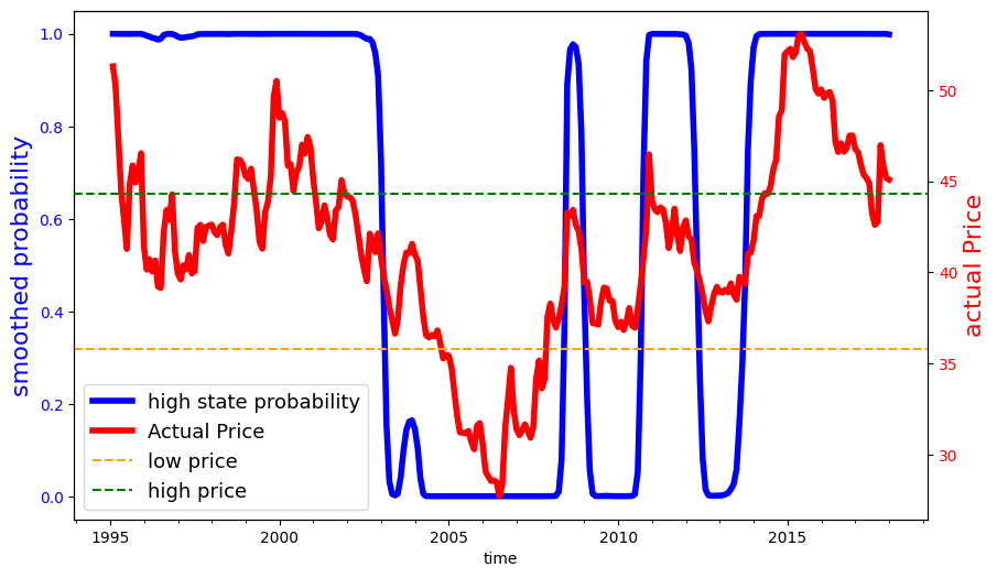
Fig. 4.1 Fig: Smoothed probabilities for distinct variances#
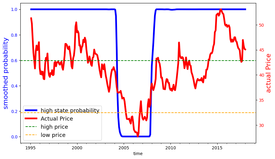
Fig. 4.2 Fig: Smoothed probabilities for common variances#
4.3.2. Optimization#
Below is the function for MPC robustness optimization. Similarly we compute the implied shadow price first and then compute the social valuations using the implied uncertainty-adjusted probability measures. To construct the business-as-usual price for emissions when the agricultural prices are stochastic, we used the smoothed probabilities reported above to assign the discrete states in our computations. While we used a probability .5 threshold for this assignment, many of the probabilities are actually close to zero or one.
import math
import time
from dataclasses import dataclass
import pandas as pd
import numpy as np
import pyomo.environ as pyo
import os
from pyomo.environ import (
    ConcreteModel,
    Constraint,
    NonNegativeReals,
    Objective,
    Param,
    RangeSet,
    Var,
    maximize,
    Set,
)
from pyomo.opt import SolverFactory
from ..services.file_service import get_path

@dataclass
class PlannerSolution:
    Z: np.ndarray
    X: np.ndarray
    U: np.ndarray
    V: np.ndarray


def mpc_solve_planner_problem(
    x0,
    z0,
    zbar,
    gamma,
    theta,
    dt=1,
    time_horizon=200,
    price_emissions=20.76,
    price_cattle=44.75,
    price_low = 35.71,
    price_high = 44.25,
    alpha=0.045007414,
    delta=0.02,
    kappa=2.094215255,
    zeta_u=1.66e-4 * 1e9,
    zeta_v=1.00e-4 * 1e9,
    solver="gurobi",
    sto_horizon=8,
    xi=10000,
    prob_ll=0.706,
    prob_hh=0.829,
    id=1,
    max_iter=20000,
    tol=0.005,
    final_sample_size=5_000,
    forest_area_2017=None,
    weight=0.5,
    low_smart_guess=None,
    high_smart_guess=None,
    mode=None,
    type=None,
):


    output_base_path = os.path.join(
        str(get_path("output")),
        "sampling",
        solver,
        f"78sites",
        f"mpc",
        f"xi_{xi}",
        f"id_{id}",
        f"pe_{price_emissions}",
    )
    if not os.path.exists(output_base_path):
        os.makedirs(output_base_path)

    model = ConcreteModel()

    # Indexing sets for time and sites
    model.T = RangeSet(time_horizon + 1)
    model.S = RangeSet(gamma.size)
    model.J = RangeSet(sto_horizon)

    # Parameters
    model.x0 = Param(model.S, initialize=_np_to_dict(x0))
    model.z0 = Param(model.S, initialize=_np_to_dict(z0))
    model.zbar = Param(model.S, initialize=_np_to_dict(zbar))
    model.gamma = Param(model.S, initialize=_np_to_dict(gamma))
    model.theta = Param(model.S, initialize=_np_to_dict(theta))
    model.delta = Param(initialize=delta)
    model.pe = Param(initialize=price_emissions)


    model.pa_current = Param(initialize=1, mutable=True)
    def initialize_pa(model,  t, j):
        if t == 1:
            return price_low if model.pa_current.value == 1 else price_high
        elif t == 2:
            if j in [1, 2, 3, 4]:
                return price_low
            else:
                return price_high
        elif t == 3:
            if j in [1, 2] or j in [5, 6]:
                return price_low
            else:
                return price_high
        elif t == 4:
            if j in [1, 3, 5, 7]:
                return price_low
            else:
                return price_high
        else:
            if j in [1, 3, 5, 7]:
                return price_low
            else:
                return price_high
    model.pa = Param(model.T, model.J, mutable=True, initialize=initialize_pa)
    # model.prob = Param(model.J, initialize=0, mutable=True)


    dep = [
        (1, 2, 1), (1, 3, 1), (1, 4, 1), (1, 5, 1), (1, 6, 1), (1, 7, 1), (1, 8, 1),
        (2, 2, 1), (2, 3, 1), (2, 4, 1), (2, 6, 2), (2, 7, 2), (2, 8, 2),
        (3, 2, 1), (3, 4, 3), (3, 6, 5), (3, 8, 7),
    ]

    model.dep = Set(initialize=dep, dimen=3)


    model.zeta_u = Param(initialize=zeta_u)
    model.zeta_v = Param(initialize=zeta_v)

    model.alpha = Param(initialize=alpha)
    model.kappa = Param(initialize=kappa)
    model.xi = Param(initialize=xi)
    model.dt = Param(initialize=dt)


    model.p_C0_1 = Param(initialize=prob_ll, mutable=True)
    model.p_C1_1 = Param(initialize=prob_ll, mutable=True)
    model.p_C1_2 = Param(initialize=prob_ll, mutable=True)
    model.p_C2_1 = Param(initialize=prob_ll, mutable=True)
    model.p_C2_2 = Param(initialize=prob_ll, mutable=True)
    model.p_C2_3 = Param(initialize=prob_ll, mutable=True)
    model.p_C2_4 = Param(initialize=prob_ll, mutable=True)

    # Variables
    model.x = Var(model.T, model.S, model.J)
    model.z = Var(model.T, model.S, model.J, within=NonNegativeReals)
    model.u = Var(model.T, model.S, model.J, within=NonNegativeReals)
    model.v = Var(model.T, model.S, model.J, within=NonNegativeReals)

    # Auxilary variables
    model.w1 = Var(model.T,model.J)
    model.w2 = Var(model.T,model.J)

    # Constraints
    model.zdot_def = Constraint(model.T, model.S,model.J, rule=_zdot_const)
    model.xdot_def = Constraint(model.T, model.S,model.J, rule=_xdot_const)
    model.w1_def = Constraint(model.T, model.J,rule=_w1_const)
    model.w2_def = Constraint(model.T, model.J,rule=_w2_const)


    model.non_x_def = Constraint(
        model.dep,
        model.S,
        rule=non_x_def_rule
    )

    model.non_z_def = Constraint(
        model.dep,
        model.S,
        rule=non_z_def_rule
    )

    model.non_u_def = Constraint(
        model.dep,
        model.S,
        rule=non_u_def_rule
    )

    model.non_v_def = Constraint(
        model.dep,
        model.S,
        rule=non_v_def_rule
    )

    model.non_w_def = Constraint(
        model.dep,
        rule=non_w_def_rule
    )


    # Define the objective
    model.obj = Objective(rule=_planner_obj, sense=maximize)

    Z, X, U, V = [], [], [], []
    Z.append(np.array([model.z0[r] for r in model.S]))
    X.append(np.array([model.x0[r] for r in model.S]))


    if type == "constrained":
        file_path = (
            get_path("output", "simulation", "mpc_path","baseline","constrained") / f"mc_{id}.csv"
        )
        print("constrained price used")
    else:
        file_path = (
            get_path("output", "simulation", "mpc_path","baseline","unconstrained") / f"mc_{id}.csv"
        )
        print("unconstrained price used")


    if mode =="converge":
        if type == "constrained":
            file_path = (
                get_path("output", "simulation", "mpc_path","constrained",f"xi_{xi}",f"pe_{price_emissions}") / f"mc_{id}.csv"
            )
        else:
            file_path = (
                get_path("output", "simulation", "mpc_path","unconstrained",f"xi_{xi}",f"pe_{price_emissions}") / f"mc_{id}.csv"
            )


    if file_path is None:
        raise ValueError(f"Invalid mode '{mode}' or price_low '{price_low}'. Could not determine file_path.")


    pa_list = np.array(pd.read_csv(file_path))[:,1]


    results = dict(
        tol=tol,
        T=model.T,
        delta_t=delta,
        alpha=alpha,
        kappa=kappa,
        pf=price_emissions,
        xi=xi,
    )

    iteration_period=time_horizon
    if mode=="sp":
        iteration_period=21


    for Q in range(iteration_period):


        model.pa_current.set_value(pa_list[Q])

        for t in model.T:
            for j in model.J:
                model.pa[t, j] = initialize_pa(model, t, j)

        print(f"Time {Q+1}: {model.pa_current.value}")


        for j in model.J:
            for s in model.S:
                model.z[:, s,j].setub(model.zbar[s])
                model.u[max(model.T), s,j].fix(0)
                model.v[max(model.T), s,j].fix(0)
                model.w1[max(model.T),j].fix(0)
                model.w2[max(model.T),j].fix(0)

                if Q ==0:
                    model.x[min(model.T), s,j].fix(model.x0[s])
                    model.z[min(model.T), s,j].fix(model.z0[s])
                if Q >0:
                    model.x[min(model.T), s,j].fix(model.x[2, s,1])
                    model.z[min(model.T), s,j].fix(model.z[2, s,1])

        # Initialize error & iteration counter
        pct_error = np.infty
        cntr = 0

        uncertain_vals_tracker = []
        pct_error_tracker = []

        # initialization


        model.p_C1_1.value = prob_ll
        model.p_C1_2.value = 1-prob_hh
        model.p_C2_1.value = prob_ll
        model.p_C2_2.value = 1-prob_hh
        model.p_C2_3.value = prob_ll
        model.p_C2_4.value = 1-prob_hh
        if model.pa_current.value == 1:
            model.p_C0_1.value = prob_ll
        if model.pa_current.value == 2:
            model.p_C0_1.value = 1-prob_hh


        model.p_C0_1_ori = model.p_C0_1.value
        model.p_C1_1_ori = model.p_C1_1.value
        model.p_C1_2_ori = model.p_C1_2.value
        model.p_C2_1_ori = model.p_C2_1.value
        model.p_C2_2_ori = model.p_C2_2.value
        model.p_C2_3_ori = model.p_C2_3.value
        model.p_C2_4_ori = model.p_C2_4.value


        if Q>0 :
            if model.pa_current.value == 1 and low_smart_guess is not None:

                (model.p_C0_1.value,model.p_C1_1.value,model.p_C1_2.value,model.p_C2_1.value,model.p_C2_2.value,model.p_C2_3.value,model.p_C2_4.value) = low_smart_guess

            if model.pa_current.value == 2 and high_smart_guess is not None:

                (model.p_C0_1.value,model.p_C1_1.value,model.p_C1_2.value,model.p_C2_1.value,model.p_C2_2.value,model.p_C2_3.value,model.p_C2_4.value) = high_smart_guess


        uncertain_vals_old = np.array([ model.p_C0_1.value, model.p_C1_1.value,model.p_C1_2.value,model.p_C2_1.value,model.p_C2_2.value,model.p_C2_3.value,model.p_C2_4.value]).copy()
        uncertain_vals =  np.array([ model.p_C0_1.value, model.p_C1_1.value,model.p_C1_2.value,model.p_C2_1.value,model.p_C2_2.value,model.p_C2_3.value,model.p_C2_4.value]).copy()


        while cntr < max_iter and pct_error > tol:
            print(f"Optimization Iteration[{cntr+1}/{max_iter}]\n")


            # Solve the model
            opt = SolverFactory(solver)
            print("Solving the optimization problem...")
            start_time = time.time()
            if solver == "gams":
                opt.solve(model, tee=True, solver="cplex", mtype="qcp")
            else:
                opt.options['Threads'] = 8
                opt.solve(model, tee=True)

            print(f"Done! Time elapsed: {time.time()-start_time} seconds.")

            g_0_1, g_1_1, g_1_2, g_2_1, g_2_2, g_2_3, g_2_4=adjust(model,T=time_horizon,S=gamma.size,J=sto_horizon)

            print("g_0_1:",g_0_1)
            print("g_1_1:",g_1_1)
            print("g_1_2:",g_1_2)
            print("g_2_1:",g_2_1)
            print("g_2_2:",g_2_2)
            print("g_2_3:",g_2_3)
            print("g_2_4:",g_2_4)

            model.p_C0_1.value = min(g_0_1*model.p_C0_1_ori,0.999)
            model.p_C1_1.value = min(g_1_1*model.p_C1_1_ori,0.999)
            model.p_C1_2.value = min(g_1_2*model.p_C1_2_ori,0.999)
            model.p_C2_1.value = min(g_2_1*model.p_C2_1_ori,0.999)
            model.p_C2_2.value = min(g_2_2*model.p_C2_2_ori,0.999)
            model.p_C2_3.value = min(g_2_3*model.p_C2_3_ori,0.999)
            model.p_C2_4.value = min(g_2_4*model.p_C2_4_ori,0.999)

            uncertain_vals = np.array([model.p_C0_1.value, model.p_C1_1.value,model.p_C1_2.value,model.p_C2_1.value,model.p_C2_2.value,model.p_C2_3.value,model.p_C2_4.value]).copy()

            print(f"Parameters from last iteration: {uncertain_vals_old}\n")
            print(
                f"""Parameters from current iteration:
                {uncertain_vals}\n"""
            )


            uncertain_vals_tracker.append(uncertain_vals.copy())

            pct_error = np.max(
                np.abs(uncertain_vals_old - uncertain_vals) / uncertain_vals_old
            )

            pct_error_tracker.append(pct_error)

            print(
                f"""
                Percentage Error = {pct_error}
                """
            )

            # Exchange parameter values
            uncertain_vals_old = uncertain_vals

            # Increase the counter
            cntr += 1

            # Update results directory
            results.update(
                {   "time_period":Q+1,
                    "cntr": cntr,
                    "pct_error_tracker": np.asarray(pct_error_tracker),
                    "uncertain_vals_tracker": np.asarray(uncertain_vals_tracker),
                }
            )


        if model.pa_current.value == 2:
            high_smart_guess=uncertain_vals
        if model.pa_current.value == 1:
            low_smart_guess=uncertain_vals


        Z.append(np.array([model.z[2, r,1].value  for r in model.S]))
        X.append(np.array([model.x[2, r,1].value  for r in model.S]))
        U.append(np.array([model.u[1, r,1].value  for r in model.S]))
        V.append(np.array([model.v[1, r,1].value  for r in model.S]))

        print("year done:",Q+1)


    Z = np.array(Z)
    X = np.array(X)
    U = np.array(U)
    V = np.array(V)


    return PlannerSolution(Z, X, U, V)


def vectorize_trajectories(traj: PlannerSolution):
    Z = traj.Z.T
    U = traj.U[:-1, :].T
    V = traj.V[:-1, :].T
    return {
        "Z": Z,
        "U": U,
        "V": V,
    }


def _zdot_const(model, t, s,j):
    if t < max(model.T):
        return (model.z[t + 1, s,j] - model.z[t, s,j]) / model.dt == (
            model.u[t, s,j] - model.v[t, s,j]
        )
    else:
        return Constraint.Skip


def _xdot_const(model, t, s,j):
    if t < max(model.T):
        return (model.x[t + 1, s,j] - model.x[t, s,j]) / model.dt == (
            -model.gamma[s] * model.u[t, s,j]
            - model.alpha * model.x[t, s,j]
            + model.alpha * model.gamma[s] * (model.zbar[s] - model.z[t, s,j])
        )
    else:
        return Constraint.Skip


def _w1_const(model, t,j):
    if t < max(model.T):
        return model.w1[t,j] == pyo.quicksum(model.u[t, s,j] for s in model.S)
    else:
        return Constraint.Skip


def _w2_const(model, t,j):
    if t < max(model.T):
        return model.w2[t,j] == pyo.quicksum(model.v[t, s,j] for s in model.S)
    else:
        return Constraint.Skip


def _np_to_dict(x):
    return dict(enumerate(x.flatten(), 1))


def non_x_def_rule(model, t, j, j1, s):
    return model.x[t+1, s, j] == model.x[t+1, s, j1]

def non_z_def_rule(model, t, j, j1, s):
    return model.z[t+1,s, j] == model.z[ t+1,s, j1]


def non_u_def_rule(model, t, j, j1, s):
    return model.u[t,s, j] == model.u[ t,s, j1]


def non_v_def_rule(model, t, j, j1, s):
    return model.v[t,s, j] == model.v[ t,s, j1]

def non_w_def_rule(model, t, j, j1):
    return model.w1[t,j] == model.w1[ t,j1]


def _planner_obj(model):

    def compute_flow(model, t, j):
        return (
            -model.pe
            * pyo.quicksum(
                model.kappa * model.z[t + 1, s, j]
                - (model.x[t + 1, s, j] - model.x[t, s, j]) / model.dt
                for s in model.S
            )
            + model.pa[t, j]
            * pyo.quicksum(model.theta[s] * model.z[t + 1, s, j] for s in model.S)
            - (model.zeta_u / 2) * (model.w1[t, j] ** 2)
            - (model.zeta_v / 2) * (model.w2[t, j] ** 2)
        )


    object_value_C_t3 = {
        j: (1 - math.exp(-model.delta)) * pyo.quicksum(
            math.exp(-model.delta * (t * model.dt - 4 * model.dt)) *
            compute_flow(model, t, j) * model.dt
            for t in model.T
            if t < max(model.T) and t > 3
        )
        for j in model.J
    }


    # Group states into state primes: {1, 2}, {3, 4}, {5, 6}, {7, 8}
    state_C2_C3_mapping = {
        1: [1, 2],
        2: [1, 2],
        3: [3, 4],
        4: [3, 4],
        5: [5, 6],
        6: [5, 6],
        7: [7, 8],
        8: [7, 8],
    }

    state_C2_C3_prob = {
        1: model.p_C2_1,
        2: 1-model.p_C2_1,
        3: model.p_C2_2,
        4: 1-model.p_C2_2,
        5: model.p_C2_3,
        6: 1-model.p_C2_3,
        7: model.p_C2_4,
        8: 1-model.p_C2_4,
    }


    object_value_C_t2 = {
        j: (1 - pyo.exp(-model.delta)) *  compute_flow(model, 3, j)
        + pyo.exp(-model.delta) * pyo.quicksum(
            state_C2_C3_prob[mapping] * object_value_C_t3[mapping]
            for mapping in state_C2_C3_mapping[j]
        )
        for j in model.J
    }


    state_C1_C2_prob = {
        1: model.p_C1_1,
        2: model.p_C1_1,
        3: 1-model.p_C1_1,
        4: 1-model.p_C1_1,
        5: model.p_C1_2,
        6: model.p_C1_2,
        7: 1-model.p_C1_2,
        8: 1-model.p_C1_2,
    }

    object_value_C_t1_unique = {}

    object_value_C_t1_unique[0] = (
        (1 - pyo.exp(-model.delta)) *  compute_flow(model, 2, 1)
        + pyo.exp(-model.delta) *  pyo.quicksum(
            state_C1_C2_prob[j] * object_value_C_t2[j]
            for j in [1, 3]
        )
    )

    object_value_C_t1_unique[1] = (
        (1 - pyo.exp(-model.delta)) * compute_flow(model, 2, 5)
        + pyo.exp(-model.delta) *  pyo.quicksum(
            state_C1_C2_prob[j] * object_value_C_t2[j]
            for j in [5, 7]
        )
    )


    object_value_C_t0 = (
        (1 - pyo.exp(-model.delta)) *  compute_flow(model, 1, 1)
        + pyo.exp(-model.delta) * (
            model.p_C0_1 * object_value_C_t1_unique[0]
            + (1-model.p_C0_1) * object_value_C_t1_unique[1]
        )
    )


    return object_value_C_t0


def adjust(model,T,S,J):


    dt = model.dt.value
    delta = model.delta.value
    pe = model.pe.value
    kappa = model.kappa.value
    zeta_u = model.zeta_u.value
    zeta_v = model.zeta_v.value
    xi = model.xi.value

    z = np.array([[[model.z[t, r, j].value for t in model.T] for r in model.S] for j in model.J])  # Shape: (J, S, T + 1)
    x = np.array([[[model.x[t, r, j].value for t in model.T] for r in model.S] for j in model.J])
    pa = np.array([[model.pa[t, j].value for t in model.T] for j in model.J])
    theta = np.array([model.theta[s] for s in model.S])
    w1 = np.array([[model.w1[t, j].value for t in model.T] for j in model.J])
    w2 = np.array([[model.w2[t, j].value for t in model.T] for j in model.J])


    def compute_flow2(t, j):
        dz = z[j, :, t+1]
        dx = (x[j, :, t+1] - x[j, :, t]) / dt
        flow = (
            -pe * np.sum(kappa * dz - dx)
            + pa[j, t] * np.sum(theta * dz)
            - (zeta_u / 2) * (w1[j, t] ** 2)
            - (zeta_v / 2) * (w2[j, t] ** 2)
        )
        return flow


    object_value_C_t3 = {}
    for j in range(J):
        object_value_C_t3[j+1] = (1 - np.exp(-delta)) * sum(
            np.exp(-delta * (t * dt - 3 * dt)) * compute_flow2(t, j)
            for t in range(3, T)
        ) * dt


    g_2_1= np.exp(-1/xi*object_value_C_t3[1])/(model.p_C2_1_ori*np.exp(-1/xi*object_value_C_t3[1])+(1-model.p_C2_1_ori)*np.exp(-1/xi*object_value_C_t3[2]))
    g_2_2= np.exp(-1/xi*object_value_C_t3[3])/(model.p_C2_2_ori*np.exp(-1/xi*object_value_C_t3[3])+(1-model.p_C2_2_ori)*np.exp(-1/xi*object_value_C_t3[4]))
    g_2_3= np.exp(-1/xi*object_value_C_t3[5])/(model.p_C2_3_ori*np.exp(-1/xi*object_value_C_t3[5])+(1-model.p_C2_3_ori)*np.exp(-1/xi*object_value_C_t3[6]))
    g_2_4= np.exp(-1/xi*object_value_C_t3[7])/(model.p_C2_4_ori*np.exp(-1/xi*object_value_C_t3[7])+(1-model.p_C2_4_ori)*np.exp(-1/xi*object_value_C_t3[8]))


    # Group states into state primes: {1, 2}, {3, 4}, {5, 6}, {7, 8}
    state_C2_C3_mapping = {
        1: [1, 2],
        2: [1, 2],
        3: [3, 4],
        4: [3, 4],
        5: [5, 6],
        6: [5, 6],
        7: [7, 8],
        8: [7, 8],
    }

    state_C2_C3_prob = {
        1: model.p_C2_1_ori,
        2: 1-model.p_C2_1_ori,
        3: model.p_C2_2_ori,
        4: 1-model.p_C2_2_ori,
        5: model.p_C2_3_ori,
        6: 1-model.p_C2_3_ori,
        7: model.p_C2_4_ori,
        8: 1-model.p_C2_4_ori,
    }


    object_value_C_t2 = {
        j+1: (1 - np.exp(-delta)) * compute_flow2(2, j)
        - np.exp(-delta) * xi * np.log(sum(
            state_C2_C3_prob[m] * np.exp(-1/xi*object_value_C_t3[m]) for m in state_C2_C3_mapping[j+1]
        ))
        for j in range(J)
    }


    g_1_1 = np.exp(-1/xi*object_value_C_t2[1])/(model.p_C1_1_ori*np.exp(-1/xi*object_value_C_t2[1])+(1-model.p_C1_1_ori)*np.exp(-1/xi*object_value_C_t2[3]))
    g_1_2 = np.exp(-1/xi*object_value_C_t2[5])/(model.p_C1_2_ori*np.exp(-1/xi*object_value_C_t2[5])+(1-model.p_C1_2_ori)*np.exp(-1/xi*object_value_C_t2[7]))


    state_C1_C2_prob = {
        1: model.p_C1_1_ori,
        2: model.p_C1_1_ori,
        3: 1-model.p_C1_1_ori,
        4: 1-model.p_C1_1_ori,
        5: model.p_C1_2_ori,
        6: model.p_C1_2_ori,
        7: 1-model.p_C1_2_ori,
        8: 1-model.p_C1_2_ori,
    }

    obj_C_t1 = {}
    obj_C_t1[0] = (1 - np.exp(-delta)) * compute_flow2(1, 0) - np.exp(-delta) * xi * np.log( sum(
        state_C1_C2_prob[j] * np.exp(-1/xi*object_value_C_t2[j]) for j in [1,3]
    ))
    obj_C_t1[1] = (1 - np.exp(-delta)) * compute_flow2(1, 4) - np.exp(-delta) * xi * np.log( sum(
        state_C1_C2_prob[j] * np.exp(-1/xi*object_value_C_t2[j]) for j in [5,7]
    ))


    g_0_1 = np.exp(-1/xi*obj_C_t1[0])/(model.p_C0_1_ori*np.exp(-1/xi*obj_C_t1[0])+(1-model.p_C0_1_ori)*np.exp(-1/xi*obj_C_t1[1]))


    return g_0_1, g_1_1, g_1_2, g_2_1, g_2_2, g_2_3, g_2_4
number of sites |
agricultural price |
\(\xi\) |
carbon price (\(P^{ee}\)) |
|---|---|---|---|
78 |
stochastic |
\(\infty\) |
6.3 |
78 |
stochastic |
1 |
6.0 |
78 |
stochastic |
0.5 |
5.6 |
Show code cell source
import pandas as pd
import numpy as np
import os
import ipywidgets as widgets
from IPython.display import display, HTML
from IPython.display import display, Math, Latex
root_folder='/project/lhansen/HMC_book/Amazon/docs'
os.chdir(root_folder)

def rename(df):
    df.columns = ['ξ̂', 'agricultural output', 'net transfers',
                'forest services', 'adjustment costs', 'planner value']
    # Define the custom values for the first row
    custom_values = [''] + ['($10^11)'] * 5

    # Create a new DataFrame for the new row with the custom values
    new_row = pd.DataFrame([custom_values], columns=df.columns)

    # Concatenate this new row to the top of the existing DataFrame
    df = pd.concat([new_row, df], ignore_index=True)

    return df
# Example DataFrames for Model A and Model B
df_mpc_b0=pd.read_csv(os.getcwd()+'/data/78site/mpc/mpc_b0.csv',na_filter=False)
df_mpc_b0 = rename(df_mpc_b0)
df_mpc_b10=pd.read_csv(os.getcwd()+'/data/78site/mpc/mpc_b10.csv',na_filter=False)
df_mpc_b10 = rename(df_mpc_b10)
df_mpc_b15=pd.read_csv(os.getcwd()+'/data/78site/mpc/mpc_b15.csv',na_filter=False)
df_mpc_b15 = rename(df_mpc_b15)
df_mpc_b25=pd.read_csv(os.getcwd()+'/data/78site/mpc/mpc_b25.csv',na_filter=False)
df_mpc_b25 = rename(df_mpc_b25)

def create_df_widget(df,subtitle,tag_id):
    """Utility function to create a widget for displaying a DataFrame with centered cells."""
    # Define CSS to center text in table cells
    style = """
    <style>
        .dataframe td, .dataframe th {
            text-align: center;
            vertical-align: middle;
        }
        .dataframe thead th {
            background-color: #f2f2f2;  # Light gray background in the header
        }
    </style>
    """
    # Convert DataFrame to HTML and manually add the 'id' attribute
    html_df = df.to_html(index=False, escape=False)
    html_df = html_df.replace('<table border="1" class="dataframe">', f'<table id="{tag_id}" border="1" class="dataframe">')

    html = style + html_df
    html_widget = widgets.HTML(value=html)  # Use ipywidgets.HTML here
    subtitle_widget = widgets.Label(value=subtitle, layout=widgets.Layout(justify_content='center'))
    out = widgets.VBox([subtitle_widget, html_widget], layout={'border': '1px solid black'})
    return out


# Tab widget to hold different models
tab = widgets.Tab()
children = [create_df_widget(df_mpc_b0,'Present-value decomposition - price stochasticity','tab:valueObjectiveDecomposition_1043sites_det3'),
            create_df_widget(df_mpc_b10,'Present-value decomposition - price stochasticity','tab:valueObjectiveDecomposition_1043sites_det3'),
            create_df_widget(df_mpc_b15,'Present-value decomposition - price stochasticity','tab:valueObjectiveDecomposition_1043sites_det3'),
            create_df_widget(df_mpc_b25,'Present-value decomposition - price stochasticity','tab:valueObjectiveDecomposition_1043sites_det3'),
            ]
tab.children = children
for i, title in enumerate(['b = 0 ','b = 10 ', 'b = 15', 'b = 25']):
    tab.set_title(i, title)

# Display the tab widget
tab.selected_index = 0
display(tab)
Show code cell source
import pandas as pd
import numpy as np
import os
import ipywidgets as widgets
from IPython.display import display, HTML
from IPython.display import display, Math, Latex
root_folder='/project/lhansen/HMC_book/Amazon/docs'
os.chdir(root_folder)

def rename(df):
    df.columns = ['ξ̂', 'Prob from low to low', 'Prob from high to high']

    return df
# Example DataFrames for Model A and Model B
tran_b0=pd.read_csv(os.getcwd()+'/data/78site/mpc/tran_b0.csv',na_filter=False)
tran_b0 = rename(tran_b0)
tran_b10=pd.read_csv(os.getcwd()+'/data/78site/mpc/tran_b10.csv',na_filter=False)
tran_b10 = rename(tran_b10)
tran_b15=pd.read_csv(os.getcwd()+'/data/78site/mpc/tran_b15.csv',na_filter=False)
tran_b15 = rename(tran_b15)
tran_b25=pd.read_csv(os.getcwd()+'/data/78site/mpc/tran_b25.csv',na_filter=False)
tran_b25 = rename(tran_b25)


def create_df_widget(df,subtitle,tag_id):
    """Utility function to create a widget for displaying a DataFrame with centered cells."""
    # Define CSS to center text in table cells
    style = """
    <style>
        .dataframe td, .dataframe th {
            text-align: center;
            vertical-align: middle;
        }
        .dataframe thead th {
            background-color: #f2f2f2;  # Light gray background in the header
        }
    </style>
    """
    # Convert DataFrame to HTML and manually add the 'id' attribute
    html_df = df.to_html(index=False, escape=False)
    html_df = html_df.replace('<table border="1" class="dataframe">', f'<table id="{tag_id}" border="1" class="dataframe">')

    html = style + html_df
    html_widget = widgets.HTML(value=html)  # Use ipywidgets.HTML here
    subtitle_widget = widgets.Label(value=subtitle, layout=widgets.Layout(justify_content='center'))
    out = widgets.VBox([subtitle_widget, html_widget], layout={'border': '1px solid black'})
    return out


# Tab widget to hold different models
tab = widgets.Tab()
children = [create_df_widget(tran_b0,'Uncertainty-adjusted transition probability','tab:valueObjectiveDecomposition_1043sites_det3'),
            create_df_widget(tran_b10,'Uncertainty-adjusted transition probability','tab:valueObjectiveDecomposition_1043sites_det3'),
            create_df_widget(tran_b15,'Uncertainty-adjusted transition probability','tab:valueObjectiveDecomposition_1043sites_det3'),
            create_df_widget(tran_b25,'Uncertainty-adjusted transition probability','tab:valueObjectiveDecomposition_1043sites_det3'),
            ]
tab.children = children
for i, title in enumerate(['b = 0 ','b = 10 ', 'b = 15', 'b = 25']):
    tab.set_title(i, title)

# Display the tab widget
tab.selected_index = 0
display(tab)