2. Solution with parameter ambiguity neutrality#
2.1. Model setup#
For the case with parameter ambiguity neutrality and without price stochastic, we are solving the following maximization problem, for a horizon of 200 years:
subject to the initial conditions and constraints:
where \(Z_t\) is vector of agricultural areas expressed in hectares and \(X_t\) is vector of carbon captured expressed in Mg CO2e. The state vector \(Z_t\) is subject to an instant-by-instant and coordinate-by-coordinate constraint: \( 0 \le Z_t^i \le {\bar z}^i \) where \({\bar z}^i\) is the amount of land in the Amazon biome available for agriculture at site \(i\).
We model the value of cattle output in site \(i\) as \(P_t^a A_t^i\), where \(A_t^i\) is proportional to the land allocated to cattle farming: \(A_t^i=\theta^i Z_t^i\)
To confront the inequality restrictions that are central to our problem, we use a so-called interior point method. This method imposes penalties on logarithms of variables that are constrained to be non-negative. While the interior point approximation pushes solutions away from their zero boundaries, in practice the solutions will be close enough to zero to identify the binding constraints.
2.2. Parameter setting#
\(P^e\) is the price for carbon emissions.
\(P^a\) is the price of agriculture.
\(\alpha\) is a carbon depreciation parameter, assumed to be constant across sites. It is set so that the 99% convergence time of the carbon accumulation process is 100 years (see Heinrich et al. (2021)), that is \(\alpha=1-(1-0.99)^{1/100}=.045\).
\(\kappa\) is calibrated using the agricultural net annual emission data at the state level available from the system SEEG. We use \(\kappa=2.0942,\) which is the average of agricultural net emission divided by the agricultural area from MapBiomas for all states within the Amazon biome, weighting by the area of each state overlap with the biome, from 1990 to 2019.
\(\delta\) is the discount rate.
\(\zeta\)s are adjustment costs. To calibrate \(\zeta_1\), we compute the average marginal cost of deforestation implied by our model using data from MapBiomas on annual historical deforestation between 2008 – 2017 (Souza et al., 2020) and match this to the difference in prices for forested and clear land (Araújo, Costa and Sant’Anna, 2024). To calibrate \(\zeta_2\), we compute the average marginal cost of natural reforestation using data from MapBiomas on annual historical secondary vegetation age (Souza et al., 2020) and match this to natural reforestation costs in Benini and Adeodato (2017).
## Parameter setting

dt=1,
time_horizon=200,
price_emissions=20.76,
price_cattle=44.75,
alpha=0.045007414,
delta=0.02,
kappa=2.094215255,
zeta_u=1.66e-4 * 1e9,
zeta_v=1.00e-4 * 1e9,
solver="gurobi",
2.3. Model solving#
In the code below, we construct a function to solve the social planner’s problem using \(\bf{Gurobi}\), a state-of-the-art optimization solver capable of efficiently handling a wide range of mathematical programming tasks. In this study, we primarily rely on its support for Quadratically Constrained Programming (QCP) problems. See Gurobi for more details.
import math
import time
from dataclasses import dataclass

import numpy as np
import pyomo.environ as pyo
from pyomo.environ import (
    ConcreteModel,
    Constraint,
    NonNegativeReals,
    Objective,
    Param,
    RangeSet,
    Var,
    maximize,
)
from pyomo.opt import SolverFactory


@dataclass
class PlannerSolution:
    Z: np.ndarray
    X: np.ndarray
    U: np.ndarray
    V: np.ndarray


def solve_planner_problem(
    x0,
    z0,
    zbar,
    gamma,
    theta,
    dt=1,
    time_horizon=200,
    price_emissions=20.76,
    price_cattle=44.75,
    alpha=0.045007414,
    delta=0.02,
    kappa=2.094215255,
    zeta_u=1.66e-4 * 1e9,
    zeta_v=1.00e-4 * 1e9,
    solver="gurobi",
):
    model = ConcreteModel()

    # Indexing sets for time and sites
    model.T = RangeSet(time_horizon + 1)
    model.S = RangeSet(gamma.size)

    # Parameters
    model.x0 = Param(model.S, initialize=_np_to_dict(x0))
    model.z0 = Param(model.S, initialize=_np_to_dict(z0))
    model.zbar = Param(model.S, initialize=_np_to_dict(zbar))
    model.gamma = Param(model.S, initialize=_np_to_dict(gamma))
    model.theta = Param(model.S, initialize=_np_to_dict(theta))
    model.delta = Param(initialize=delta)
    model.pe = Param(initialize=price_emissions)

    # Set cattle price as series
    if isinstance(price_cattle, float):
        price_cattle = {t + 1: price_cattle for t in range(time_horizon)}
    else:
        price_cattle = {t + 1: price_cattle[t] for t in range(time_horizon)}

    model.pa = Param(model.T, initialize=price_cattle)

    # Asymmetric adj. costs
    model.zeta_u = Param(initialize=zeta_u)
    model.zeta_v = Param(initialize=zeta_v)

    model.alpha = Param(initialize=alpha)
    model.kappa = Param(initialize=kappa)
    model.dt = Param(initialize=dt)

    # Variables
    model.x = Var(model.T, model.S)
    model.z = Var(model.T, model.S, within=NonNegativeReals)
    model.u = Var(model.T, model.S, within=NonNegativeReals)
    model.v = Var(model.T, model.S, within=NonNegativeReals)

    # Auxilary variables
    model.w1 = Var(model.T)
    model.w2 = Var(model.T)

    # Constraints
    model.zdot_def = Constraint(model.T, model.S, rule=_zdot_const)
    model.xdot_def = Constraint(model.T, model.S, rule=_xdot_const)
    model.w1_def = Constraint(model.T, rule=_w1_const)
    model.w2_def = Constraint(model.T, rule=_w2_const)

    # Define the objective
    model.obj = Objective(rule=_planner_obj, sense=maximize)

    # Initial and terminal conditions
    for s in model.S:
        model.z[:, s].setub(model.zbar[s])
        model.x[min(model.T), s].fix(model.x0[s])
        model.z[min(model.T), s].fix(model.z0[s])
        model.u[max(model.T), s].fix(0)
        model.v[max(model.T), s].fix(0)
        model.w1[max(model.T)].fix(0)
        model.w2[max(model.T)].fix(0)

    # Solve the model
    opt = SolverFactory(solver)
    print("Solving the optimization problem...")
    start_time = time.time()
    if solver == "gams":
        opt.solve(model, tee=True, solver="cplex", mtype="qcp")
    else:
        opt.solve(model, tee=True)

    print(f"Done! Time elapsed: {time.time()-start_time} seconds.")

    Z = np.array([[model.z[t, r].value for r in model.S] for t in model.T])
    X = np.array([[model.x[t, r].value for r in model.S] for t in model.T])
    U = np.array([[model.u[t, r].value for r in model.S] for t in model.T])
    V = np.array([[model.v[t, r].value for r in model.S] for t in model.T])

    return PlannerSolution(Z, X, U, V)


def vectorize_trajectories(traj: PlannerSolution):
    Z = traj.Z.T
    U = traj.U[:-1, :].T
    V = traj.V[:-1, :].T
    return {
        "Z": Z,
        "U": U,
        "V": V,
    }


def _planner_obj(model):
    return pyo.quicksum(
        math.exp(-model.delta * (t * model.dt - model.dt))
        * (
            -model.pe
            * pyo.quicksum(
                model.kappa * model.z[t + 1, s]
                - (model.x[t + 1, s] - model.x[t, s]) / model.dt
                for s in model.S
            )
            + model.pa[t]
            * pyo.quicksum(model.theta[s] * model.z[t + 1, s] for s in model.S)
            - (model.zeta_u / 2) * (model.w1[t] ** 2)
            - (model.zeta_v / 2) * (model.w2[t] ** 2)
        )
        * model.dt
        for t in model.T
        if t < max(model.T)
    )


def _zdot_const(model, t, s):
    if t < max(model.T):
        return (model.z[t + 1, s] - model.z[t, s]) / model.dt == (
            model.u[t, s] - model.v[t, s]
        )
    else:
        return Constraint.Skip


def _xdot_const(model, t, s):
    if t < max(model.T):
        return (model.x[t + 1, s] - model.x[t, s]) / model.dt == (
            -model.gamma[s] * model.u[t, s]
            - model.alpha * model.x[t, s]
            + model.alpha * model.gamma[s] * (model.zbar[s] - model.z[t, s])
        )
    else:
        return Constraint.Skip


def _w1_const(model, t):
    if t < max(model.T):
        return model.w1[t] == pyo.quicksum(model.u[t, s] for s in model.S)
    else:
        return Constraint.Skip


def _w2_const(model, t):
    if t < max(model.T):
        return model.w2[t] == pyo.quicksum(model.v[t, s] for s in model.S)
    else:
        return Constraint.Skip


def _np_to_dict(x):
    return dict(enumerate(x.flatten(), 1))
2.4. Shadow price calculation#
We first infer a shadow value for the planner based on historical experience. To obtain this value, we first choose an interval \([\underline t, \bar t]\) and then select a time-invariant price for emissions, denoted by \(P^{ee},\) to match the aggregate deforestation predicted by the model at a final observation period \(\bar t.\) We let \((X_{\underline t}^o, Z_{\underline t}^o)\) denote the initial observed state vector. We also input the realized history of agricultural prices \(\{P^a_t: {\underline t}\le t \le {\bar t}\}.\) We then compute the optimal trajectory for the state variables implied by our model for alternative choices of \(P^{e}\) and find the \(P^{ee}\) that matches \(\sum_{i=1}^I (Z_{\bar t}^i - Z_{\underline t}^i)\) to the observed value of the aggregate deforestation in the period \([\underline t, \overline t]\).
We use \(\underline t=1995,\) the initial date for our price data and \(\bar t = 2008\) the announcement of the Amazon fund that would pay for preservation projects in the Amazon, using money contributed mostly by Norway. We first load the dataset starting at 1995:
(
    zbar_1995,
    z_1995,
    forest_area_1995,
    z_2008,
    theta,
    gamma,
) = load_site_data_1995(sitenum)

def load_site_data_1995(num_sites: int, norm_fac: float = 1e9):
    # Set data directory
    data_dir = get_path("data", "calibration")

    # Read data file
    file_path = data_dir / f"calibration_{num_sites}_sites.csv"
    df = pd.read_csv(file_path)

    # Extract information
    z_1995 = df["z_1995"].to_numpy()
    z_2008 = df["z_2008"].to_numpy()
    zbar_1995 = df["zbar_1995"].to_numpy()
    forest_area_1995 = df["area_forest_1995"].to_numpy()

    # Normalize Z data
    zbar_1995 /= norm_fac
    z_1995 /= norm_fac
    forest_area_1995 /= norm_fac

    (theta, gamma) = load_productivity_params(num_sites)

    print(f"Data successfully loaded from {data_dir}")
    return (
        zbar_1995,
        z_1995,
        forest_area_1995,
        z_2008,
        theta,
        gamma,
    )
We then perform a grid search for \(P^{ee}\) and identify the value that satisfies our criterion.
pe_values = np.arange(5, 8, 0.1)

results = np.array(
    [
        shadow_price_opt(
            zbar_1995,
            z_1995,
            forest_area_1995,
            z_2008,
            theta,
            gamma,
            sitenum=sitenum,
            solver=solver,
            timehzn=200,
            pa=pa,
            pe=pe,
        )
        for pe in pe_values
    ]
)

min_index = np.argmin(results)
min_result = results[min_index]
min_pe = pe_values[min_index]

def shadow_price_opt(
    zbar_1995,
    z_1995,
    forest_area_1995,
    z_2008,
    theta,
    gamma,
    sitenum=78,
    solver="gurobi",
    timehzn=200,
    pa=41.11,
    pe=7.1,
    model="det",
):

    pa_list = load_price_data()
    price_cattle = np.concatenate((pa_list, np.full(200 - len(pa_list), pa)))

    # Computing carbon absorbed in start period
    x0_vals_1995 = gamma * forest_area_1995

    # if model == "mpc":
    #     solve_planner_problem = gams.mpc_shadow_price

    results = solve_planner_problem(
        theta=theta,
        gamma=gamma,
        x0=x0_vals_1995,
        zbar=zbar_1995,
        z0=z_1995,
        price_emissions=pe,
        price_cattle=price_cattle,
        solver=solver,
    )
    Z = results.Z
    z_2008_agg = np.sum(z_2008) / 1e9
    ratio = (np.sum(Z[13]) - z_2008_agg) / z_2008_agg

    return ratio

def load_productivity_params(num_sites: int):
    data_dir = get_path("data", "calibration")
    productivity_params = pd.read_csv(data_dir / f"productivity_params_{num_sites}.csv")

    theta = productivity_params["theta_fit"]

    gamma = productivity_params["gamma_fit"]

    return (theta.to_numpy()[:,].flatten(), gamma.to_numpy()[:,].flatten())
number of sites |
agricultural price |
\(\xi\) |
carbon price (\(P^{ee}\)) |
|---|---|---|---|
1043 |
\(p^a = 41.1\) |
\(\infty\) |
6.6 |
78 |
\(p^a = 41.1\) |
\(\infty\) |
6.0 |
2.5. Results solved#
We then solve solutions to the optimization problem starting in 2017 and consider emission price \(P^e=P^{ee}+b\) for
\(b=0, 10,15, 20,\) and \(25\) where \(b\) represents transfers per ton of net captured emissions to the planner.
We first load the initial data at year 2017, as well as baseline distributions for \(\theta\) and \(\gamma\).
## Load initial data

def load_site_data(num_sites: int, year: int = 2017, norm_fac: float = 1e9):
    # Set data directory
    data_dir = get_path("data", "calibration")

    # Read data file
    file_path = data_dir / f"calibration_{num_sites}_sites.csv"
    file_path = data_dir / f"calibration_{num_sites}_sites.csv"
    df = pd.read_csv(file_path)

    # Extract information
    z = df[f"z_{year}"].to_numpy()
    zbar = df["zbar_2017"].to_numpy()
    forest_area = df[f"area_forest_{year}"].to_numpy()

    # Normalize Z and forest data
    z /= norm_fac
    zbar /= norm_fac
    forest_area /= norm_fac

    return (zbar, z, forest_area)


(
    zbar_2017,
    z_2017,
    forest_area_2017,
) = load_site_data(num_sites)

# Load baseline productivity params
(theta_vals, gamma_vals) = load_productivity_params(num_sites)

# Compute initial carbon stock
x0_vals = gamma_vals * forest_area_2017
Then solve the model for all transfer levels.
b = [0, 10, 15, 20, 25]
pe_values = [pee + bi for bi in b]
for pe in pe_values:
    results = solve_planner_problem(
        time_horizon=200,
        theta=theta_vals,
        gamma=gamma_vals,
        x0=x0_vals,
        zbar=zbar_2017,
        z0=z_2017,
        price_emissions=pe,
        price_cattle=pa,
        solver=solver,
    )

    print("Results for pe = ", pe)
    output_folder = (
        get_path("output")
        / "optimization"
        / model
        / solver
        / f"{num_sites}sites"
        / f"pa_{pa}"
        / f"pe_{pe}"
    )

    save_planner_solution(results, output_folder)
We then decompose the solved planner value into several terms and plot the land allocation trajectories in the next 50 years.
Show code cell source
import pandas as pd
import numpy as np
import os
import ipywidgets as widgets
from IPython.display import display, HTML
from IPython.display import display, Math, Latex
root_folder='/project/lhansen/HMC_book/Amazon/docs'
os.chdir(root_folder)

def rename(df):
    df.columns=['Pa','Pe','b','agricultural output','net transfers','forest services','adjustment costs','planner value']
    # Define the custom values for the first row
    custom_values = ['($)'] + ['($)'] + ['($)'] + ['($10^11)'] * (len(df.columns) - 3)

    # Create a new DataFrame for the new row with the custom values
    new_row = pd.DataFrame([custom_values], columns=df.columns)

    # Concatenate this new row to the top of the existing DataFrame
    df = pd.concat([new_row, df], ignore_index=True)

    return df
# Example DataFrames for Model A and Model B
df_det_1043 = pd.read_csv(os.getcwd()+'/data/1043site/det/pv_41.11.csv')
df_det_1043 = rename(df_det_1043)
# df_det_78_41 = pd.read_csv('data/78site/det/pv_41.11.csv')
# df_det_78_35 = pd.read_csv('data/78site/det/pv_35.71.csv')
# df_det_78_44 = pd.read_csv('data/78site/det/pv_44.26.csv')
# df_det_78 = pd.concat([df_det_78_35, df_det_78_41, df_det_78_44], ignore_index=True)
df_det_78 = pd.read_csv(os.getcwd()+'/data/78site/det/pv_41.11.csv')
df_det_78 = rename(df_det_78)
df_xi1 = pd.read_csv(os.getcwd()+'/data/78site/hmc/pv_xi1.csv')
df_xi1 = rename(df_xi1)
df_xi2 = pd.read_csv(os.getcwd()+'/data/78site/hmc/pv_xi2.csv')
df_xi2 = rename(df_xi2)
df_mpc=pd.read_csv(os.getcwd()+'/data/78site/mpc/mpc.csv',na_filter=False)


def create_df_widget(df,subtitle,tag_id):
    """Utility function to create a widget for displaying a DataFrame with centered cells."""
    # Define CSS to center text in table cells
    style = """
    <style>
        .dataframe td, .dataframe th {
            text-align: center;
            vertical-align: middle;
        }
        .dataframe thead th {
            background-color: #f2f2f2;  # Light gray background in the header
        }
    </style>
    """
    # Convert DataFrame to HTML and manually add the 'id' attribute
    html_df = df.to_html(index=False)
    html_df = html_df.replace('<table border="1" class="dataframe">', f'<table id="{tag_id}" border="1" class="dataframe">')

    html = style + html_df
    html_widget = widgets.HTML(value=html)  # Use ipywidgets.HTML here
    subtitle_widget = widgets.Label(value=subtitle, layout=widgets.Layout(justify_content='center'))
    out = widgets.VBox([subtitle_widget, html_widget], layout={'border': '1px solid black'})
    return out


# Tab widget to hold different models
tab = widgets.Tab()
children = [create_df_widget(df_det_1043,'Table 2 Present-value decomposition - 1043 sites','tab:valueObjectiveDecomposition_1043sites_det'),
            create_df_widget(df_det_78,'Table 4 Present-value decomposition - 78 sites','tab:valueObjectiveDecomposition_1043sites_det2')
            ]
tab.children = children
for i, title in enumerate(['1043site ξ = ∞ ','78site ξ = ∞ ']):
    tab.set_title(i, title)

# Display the tab widget
tab.selected_index = 0
display(tab)
Show code cell source
import pandas as pd
import os
import plotly.figure_factory as ff
import numpy as np
import plotly.graph_objects as go
import seaborn as sns
import matplotlib.pyplot as plt

root_folder='/project/lhansen/HMC_book/Amazon/docs'
current_folder = root_folder+"/data/1043site"
#pa_values = [ 41.11, 35.71,44.26]  # Example pa values
pa_values = [41.11]

b = [0, 10, 15, 20, 25]

colors = ['red', 'green', 'blue', 'purple', 'cyan']
df_ori=pd.read_csv(current_folder+'/hmc_1043SitesModel.csv')
dfz_bar= df_ori['zbar_2017_1043Sites']
dfz_bar_np=dfz_bar.to_numpy()

fig = go.Figure()

# Load data for each pa and add to the plot as a separate trace
for idx, pa in enumerate(pa_values):
    if pa==41.11:
        pee=6.6
    elif pa==44.26:
        pee=7.8
    elif pa==35.71:
        pee=7.4
    pe = [pee + bi for bi in b]

    variable_dict = {}
    for j in range(5):
        order = j
        os.chdir(f"{current_folder}/p_a_{pa}_p_e_{pe[order]}")
        dfz = pd.read_csv('amazon_data_z.dat', delimiter='\t')
        dfz = dfz.drop('T/R ', axis=1)
        dfz_zeronp = dfz.to_numpy()
        dfx = pd.read_csv('amazon_data_x.dat', delimiter='\t')
        dfx = dfx.drop('T   ', axis=1)
        dfx_np = dfx.to_numpy()
        variable_dict[f"results_zper{j}"] = []
        variable_dict[f"results_xagg{j}"] = dfx_np[:51]
        variable_dict[f"results_xagg_100{j}"] = [i*100 for i in variable_dict[f"results_xagg{j}"]]
        for i in range(51):
            result_zper = np.sum(dfz_zeronp[i])/(np.sum(dfz_bar_np)/1e11)
            variable_dict[f"results_zper{j}"].append(result_zper)
            variable_dict[f"results_zper_100{j}"] = [i * 100 for i in variable_dict[f"results_zper{j}"]]
        is_visible = (pa == 41.11)
        fig.add_trace(
            go.Scatter(
                x=list(range(51)),
                y=variable_dict[f"results_zper_100{j}"],
                mode='lines',
                name=f'pe={pe[j]}',
                line=dict(color=colors[j], width=4),
                visible=is_visible
            )
        )

# Reset the working directory to the original folder
os.chdir(current_folder)

# Create buttons for changing the visible trace
buttons = []
for idx, pa in enumerate(pa_values):
    buttons.append(dict(
        method='update',
        label=f'pa={pa}',
        args=[{'visible': [i >= idx*5 and i < (idx+1)*5 for i in range(len(pa_values)*5)]},
              {'title': 'Figure (a) Land allocation trajectory'}]
    ))

# Update layout with buttons
fig.update_layout(
    updatemenus=[dict(
        type="buttons",
        direction="right",
        x=0.7,
        xanchor="left",
        y=1.22,
        yanchor="top",
        buttons=buttons
    )],
    title="Figure (a) Land allocation trajectory",
    xaxis_title="Years",
    yaxis_title="Z(%)",
    width=800,  # Width of the figure in pixels
    height=400  # Height of the figure in pixels
)

fig.show()
Show code cell source
import os
import pandas as pd
import numpy as np
import plotly.graph_objects as go

root_folder='/project/lhansen/HMC_book/Amazon/docs'
current_folder = root_folder+"/data/1043site"
#pa_values = [ 41.11, 35.71,44.26]  # Example pa values
pa_values=[41.11]
b = [0, 10, 15, 20, 25]

colors = ['red', 'green', 'blue', 'purple', 'cyan']
df_ori=pd.read_csv(current_folder+'/hmc_1043SitesModel.csv')
dfz_bar= df_ori['zbar_2017_1043Sites']
dfz_bar_np=dfz_bar.to_numpy()

fig = go.Figure()

# Load data for each pa and add to the plot as a separate trace
for idx, pa in enumerate(pa_values):
    if pa==41.11:
        pee=6.6
    elif pa==44.26:
        pee=7.8
    elif pa==35.71:
        pee=7.4
    pe = [pee + bi for bi in b]

    variable_dict = {}
    for j in range(5):
        order = j
        os.chdir(f"{current_folder}/p_a_{pa}_p_e_{pe[order]}")
        dfz = pd.read_csv('amazon_data_z.dat', delimiter='\t')
        dfz = dfz.drop('T/R ', axis=1)
        dfz_zeronp = dfz.to_numpy()
        dfx = pd.read_csv('amazon_data_x.dat', delimiter='\t')
        dfx = dfx.drop('T   ', axis=1)
        dfx_np = dfx.to_numpy()
        variable_dict[f"results_zper{j}"] = []
        variable_dict[f"results_xagg_100{j}"] = np.round(dfx_np[:51]*100,1)
        flat_list = [item[0] for item in variable_dict[f"results_xagg_100{j}"]]
        variable_dict[f"results_xagg_100{j}"] = np.array(flat_list)
        is_visible = (pa == 41.11)
        fig.add_trace(
            go.Scatter(
                x=list(range(51)),
                y=variable_dict[f"results_xagg_100{j}"],
                mode='lines',
                name=f'pe={pe[j]}',
                line=dict(color=colors[j], width=4),
                visible=is_visible
            )
        )

# Reset the working directory to the original folder
os.chdir(current_folder)

# Create buttons for changing the visible trace
buttons = []
for idx, pa in enumerate(pa_values):
    buttons.append(dict(
        method='update',
        label=f'pa={pa}',
        args=[{'visible': [i >= idx*5 and i < (idx+1)*5 for i in range(len(pa_values)*5)]},
              {'title': 'Figure (b) carbon stock evolution'}]
    ))

# Update layout with buttons
fig.update_layout(
    updatemenus=[dict(
        type="buttons",
        direction="right",
        x=0.7,
        xanchor="left",
        y=1.22,
        yanchor="top",
        buttons=buttons
    )],
    title="Figure (b) carbon stock evolution",
    xaxis_title="Years",
    yaxis_title="X(billions CO2e)",
    width=800,  # Width of the figure in pixels
    height=400  # Height of the figure in pixels
)

fig.show()
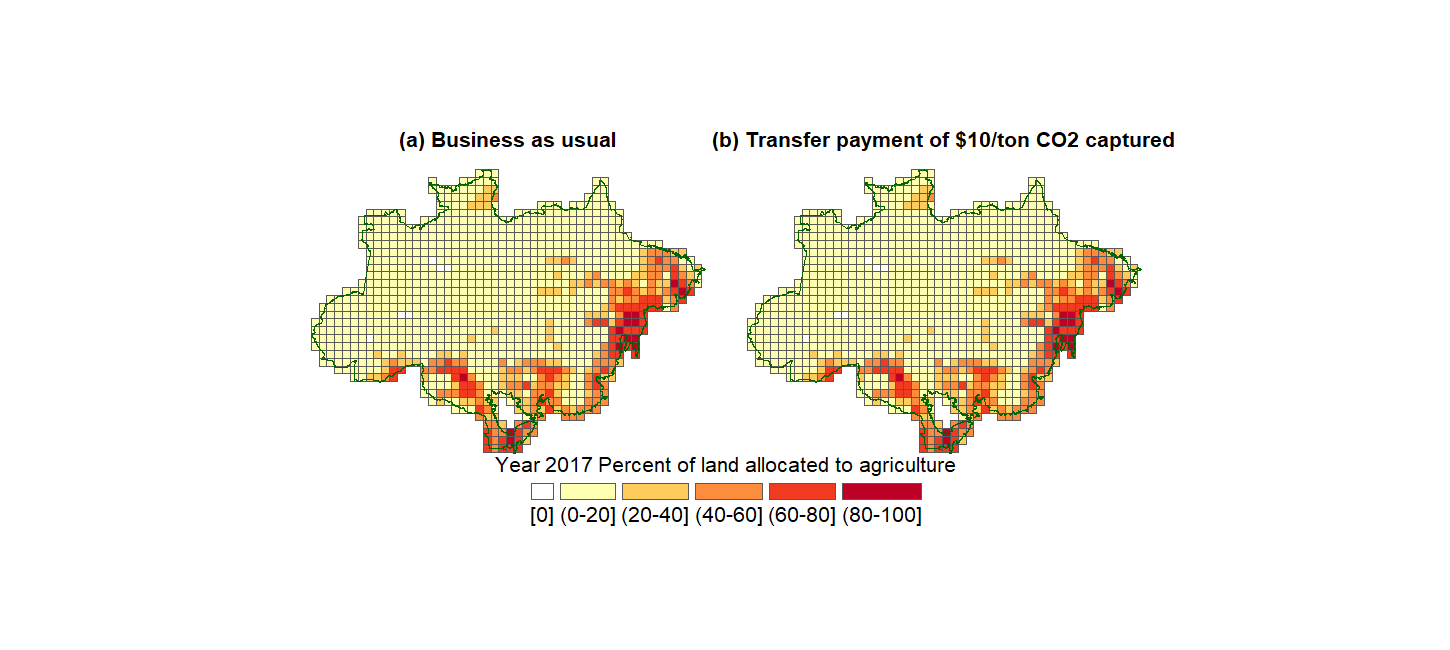
We also plot the evolution of land allocation by site until Year 2050, for the case \(b=0,10,15,20,25\).
Show code cell source
from IPython.display import HTML


HTML('''
<div style="text-align:center">
  <label><b>Select animation:</b>
    <select onchange="document.getElementById('gifImg').src=this.value">
      <option value="../_static/movie_1043site_b10.gif">  b = 10 </option>
      <option value="../_static/movie_1043site_b15.gif">  b = 15 </option>
      <option value="../_static/movie_1043site_b20.gif">  b = 20 </option>
      <option value="../_static/movie_1043site_b25.gif">  b = 25 </option>
    </select>
  </label>
  <br><br>
  <img id="gifImg" src="../_static/movie_1043site_b10.gif"
       style="border:1px solid #ccc; width:1400px; height:auto;">
</div>
''')