1. Baseline distribution

---

We start with the baseline distribution estimation for agricultural productivity parameters \(\theta\) and carbon accumulation parameter \(\gamma\). To estimate the benchmark posterior distribution \(\pi\), we consider the random effects regression models for \(\theta\) and \(\gamma\) separately. Below, we present the general specification used for these regression models, noting throughout the differences specific to the \(\theta\) and \(\gamma\) cases.

Given observations \(i=1,\ldots, N\) and groups \(b=1,\ldots, B\), we model both parameters using the following specification:

\[\begin{align*} Y = R\beta +Z\nu +U \end{align*}\]

where the observed outcome \(Y\) is N-dimensional, the vector of coefficients \(\beta\) is \(K\) dimensional, the group indicator matrix \(Z\) is \(N \times B\) dimensional, and the vector of random coefficients \(\nu\) is B-dimensional.

1.1. Load regression data

For \(\gamma\) specification, \(y^i_\gamma\) is \(\operatorname{\text{log}(CO2e\_ha)}\) and \(z^i_{\gamma}\) is the coarse site it belongs to.

\[\begin{split}\begin{align*} R^i_\gamma \beta^i_\gamma :=\; & \beta^\gamma_{0} + \beta^\gamma_{1} \log(\text{historical_precip}) + \beta^\gamma_{2} \log(\text{historical_temp}) \\ & + \beta^\gamma_{3} \text{latitude} + \beta^\gamma_{4} \text{longitude} + \beta^\gamma_{5} (\text{latitude} \times \text{longitude}) \end{align*}\end{split}\]

For \(\theta\) specification, \(y^m_{\theta}\) is \(\log(\text{Slaughter value})\) and \(z^m_{\theta}\) is Amazonian water basins.

\[\begin{split}\begin{align*} R^m_\theta \cdot \beta_\theta := \beta^\theta_{0} + \beta^\theta_{1} (\text{historical_precip}) + \beta^\theta_{2} (\text{historical_temp}) + \beta^\theta_{3} (\text{historical_temp}^2) \\ \quad + \beta^\theta_{4} (\text{lat}) + \beta^\theta_{5} (\text{lat}^2) + \beta^\theta_{6} \log(\text{cattleSlaughter_farmGatePrice}) + \beta^\theta_{7} (\text{distance}) \end{align*}\end{split}\]

In the code below, we load the regression data and fitting data separately. Note that regression data is a subset of fitting data because of missing values. We use fitting data to predict fitted values for these observations.

def load_gamma_calib(num_sites: int, type: str = "reg"):
    data_dir = get_path("data", "calibration")
    if type == "fit":
        # Used for gamma projection onto fitted values
        df = gpd.read_file(data_dir / f"gamma_fit_{num_sites}.geojson")

        # Get design matrix and its dimensions
        X = df.iloc[:, :6].to_numpy()
        N, K = X.shape

        # Large group indicator
        m = df["id_group"].astype(int)

        return {
            "X_gamma_fit": X,
            "m_gamma_fit": m,
        }
    else:
        # Used for gamma regression
        df = gpd.read_file(data_dir / "gamma_reg.geojson")

        # Get design matrix and its dimensions
        M = df["id_group"].unique().size
        y = df["log_co2e_ha_2017"]
        X = df.iloc[:, :6].to_numpy()
        N, K = X.shape

        # Large group indicator
        m = df["id_group"].astype(int)

        return {
            "N_gamma": N,
            "M_gamma": M,
            "K_gamma": K,
            "y_gamma": y,
            "X_gamma": X,
            "m_gamma": m,
        }


def load_theta_calib(num_sites: int, type: str = "reg"):
    data_dir = get_path("data", "calibration")
    if type == "fit":
        df = gpd.read_file(data_dir / f"theta_fit_{num_sites}.geojson")

        # Create the projection matrix
        G = (
            df.pivot(index="id", columns="muni_id", values="muni_site_area")
            .fillna(0)
            .to_numpy()
        )

        # Normalize to make row-stochastic
        G = G / G.sum(axis=1, keepdims=True)

        # Collapse data set to the municipality level
        df = df.sort_values("muni_id")

        # Keep first observation per municipality
        df = df.drop_duplicates(subset="muni_id", keep="first")

        # Get design matrix
        X = df.iloc[:, :8].to_numpy()
        C, _ = X.shape

        # Large group indicator
        m = df["group_id"].astype(int)

        # Cattle price in 2017
        pa_2017 = 44.9736197781184

        G_sparse = csr_matrix(G)

        # Extract CSR components
        G_w = G_sparse.data  # Non-zero values
        G_v = G_sparse.indices + 1  # Column indices
        G_u = G_sparse.indptr + 1  # Row pointers
        G_nnz = len(G_w)

        return {
            "C_theta_fit": C,
            "X_theta_fit": X,
            "m_theta_fit": m,
            "G_nnz_theta": G_nnz,
            "G_w_theta": G_w,
            "G_v_theta": G_v,
            "G_u_theta": G_u,
            "pa_2017": pa_2017,
        }

    else:
        df = gpd.read_file(data_dir / "theta_reg.geojson")
        # Get number of groups
        M = df["group_id"].unique().size

        # Get design matrix and its dimensions
        y = df["log_slaughter"]
        X = df.iloc[:, :8].to_numpy()
        N, K = X.shape

        # Large group indicator
        m = df["group_id"].astype(int)

        W = df["weights"].values
        W = np.sqrt(W / np.std(W))

        return {
            "N_theta": N,
            "M_theta": M,
            "K_theta": K,
            "y_theta": y,
            "X_theta": X,
            "m_theta": m,
            "W_theta": W,
        }


data = dict(
    num_sites=num_sites,
    **load_gamma_calib(num_sites, "reg"),
    **load_gamma_calib(num_sites, "fit"),
    **load_theta_calib(num_sites, "reg"),
    **load_theta_calib(num_sites, "fit"),
)

1.2. Fit Bayesian model

Recall the general specification:

\[\begin{align*} Y = R\beta +Z\nu +U \end{align*}\]

We model the common shock \(U\) as independent but heterogeneous:

\[U \sim \textrm{Normal} \left(0, \frac{1}{\eta}\Sigma \right),\]

where \(\Sigma\) is a diagonal matrix. Let the weighting matrix \(W\) be such that \(WW'=\Sigma^{-1}\). We then define the following density for the transformed variable \(WY\), conditional on regressors and parameters:

\[WY | W,R,Z,\beta,\nu,\eta \sim \textrm{Normal}\left( WR \beta+WZ\nu, \ \frac{1}{\eta} I \right).\]

We impose normal priors on both vectors of coefficients including the random effects, with precision parameters \(\eta\) and \(\zeta\), respectively:

\[\beta \mid \eta, \zeta \sim \textrm{Normal} \left(0, \frac 1 \eta \Omega^{-1}\right), \quad \nu \mid \eta, \zeta \sim \textrm{Normal} \left( 0, \frac 1 \zeta I \right).\]

Finally, we impose improper uniform priors on \(\log(\eta)\) and \(\log(\zeta)\), and take the limit as \(\Omega\to0\). We can then sample from the posterior density, which is proportional to the model-implied likelihood and our choice of priors:

\[ {\overline \pi}(\rho \mid W, R, Y, Z) \ \propto \ {\mathcal L}(Y|W, R, Z, \rho) \pi(\rho ),\]

For the posterior sampling, we rely on \(\bf{Stan}\), a high-performance probabilistic programming language designed for efficient Bayesian inference. See Stan for more details.

### baseline.stan ###

data {
  // Gamma regression
  int<lower=1> N_gamma; // total number of observations
  int<lower=1> K_gamma; // number of predictors
  int<lower=1> M_gamma; // number of groups
  matrix[N_gamma, K_gamma] X_gamma; // design matrix
  vector[N_gamma] y_gamma; // outcome variable
  array[N_gamma] int m_gamma; // group map

  // Theta regression
  int<lower=1> N_theta; // total number of observations
  int<lower=1> K_theta; // number of predictors
  int<lower=1> M_theta; // number of groups
  matrix[N_theta, K_theta] X_theta; // design matrix
  vector[N_theta] y_theta; // outcome variable
  array[N_theta] int m_theta; // group map
  vector[N_theta] W_theta; // weights

  // Gamma projection
  int<lower=1> num_sites; // number of samples
  matrix[num_sites, K_gamma] X_gamma_fit; // design matrix
  array[num_sites] int m_gamma_fit; // group map

  // Theta projection
  int<lower=1> C_theta_fit; // Number of municipalities
  matrix[C_theta_fit, K_theta] X_theta_fit; // design matrix
  array[C_theta_fit] int m_theta_fit; // group map

  // Sparse G_theta
  int<lower=0> G_nnz_theta; // Number of non-zero elements
  vector[G_nnz_theta] G_w_theta; // Non-zero values
  array[G_nnz_theta] int G_v_theta; // Column indices (1-based in Stan)
  array[num_sites + 1] int G_u_theta; // Row pointers (1-based in Stan)
  real pa_2017; // price of cattle in 2017
}
transformed data {
  vector[N_theta] y_theta_w = W_theta .* y_theta;
  matrix[N_theta, K_theta] X_theta_w;
  for (n in 1 : N_theta)
    X_theta_w[n] = W_theta[n] * X_theta[n];
}
parameters {
  // Gamma regression parameters
  vector[K_gamma] beta_gamma;
  vector[M_gamma] nu_gamma;
  real log_precision_u_gamma;
  real log_precision_v_gamma;

  // Theta regression parameters
  vector[K_theta] beta_theta;
  vector[M_theta] nu_theta;
  real log_precision_u_theta;
  real log_precision_v_theta;
}
transformed parameters {
  // Pre-multiply theta FE's by weights
  vector[N_theta] nu_theta_w = W_theta .* nu_theta[m_theta];
  vector[C_theta_fit] nu_theta_fit = nu_theta[m_theta_fit];
  vector[N_gamma] nu_gamma_sort = nu_gamma[m_gamma];
  vector[num_sites] nu_gamma_fit = nu_gamma[m_gamma_fit];

  real sigma_u_gamma = exp(-0.5 * log_precision_u_gamma);
  real sigma_v_gamma = exp(-0.5 * log_precision_v_gamma);
  real sigma_u_theta = exp(-0.5 * log_precision_u_theta);
  real sigma_v_theta = exp(-0.5 * log_precision_v_theta);

  // Projection
  vector<lower=0>[num_sites] gamma = exp(X_gamma_fit * beta_gamma
                                         + nu_gamma_fit);

  vector[C_theta_fit] exp_log_theta = exp(X_theta_fit * beta_theta
                                          + nu_theta_fit);

  vector<lower=0>[num_sites] theta = csr_matrix_times_vector(num_sites,
                                                             C_theta_fit,
                                                             G_w_theta,
                                                             G_v_theta,
                                                             G_u_theta,
                                                             exp_log_theta)
                                     / pa_2017;

  // for (n in 1 : N_nonzero_G_theta) {
  //   theta[row_G_theta[n]] += val_G_theta[n] * exp_log_theta[col_G_theta[n]]
  //                            / pa_2017;
  // }
}
model {
  // Priors
  nu_gamma ~ normal(0, sigma_v_gamma);
  nu_theta ~ normal(0, sigma_v_theta);

  y_gamma ~ normal(X_gamma * beta_gamma + nu_gamma_sort, sigma_u_gamma);
  y_theta_w ~ normal(X_theta_w * beta_theta + nu_theta_w, sigma_u_theta);
}

We then compile the Stan model in python and output posterior distributions

# Define output paths
output_dir = get_path("data", "calibration")
os.makedirs(get_path("output", "tables"), exist_ok=True)

# Compile Stan code
sampler = CmdStanModel(
    stan_file=get_path("stan_model") / "baseline.stan",
    cpp_options={"STAN_THREADS": "true"},
    force_compile=True,
)

# Set sampling params
stan_kwargs = dict(
    iter_sampling=1500,
    iter_warmup=500,
    show_progress=True,
    seed=1,
    inits=0.2,
    chains=4,
)

# Sampling from baseline distribution
start_time = time.time()
fit = sampler.sample(
    data=data,
    **stan_kwargs,
)
end_time = time.time()

# Compute average baseline gamma and theta
gamma_mean = fit.stan_variable("gamma").mean(axis=0)
theta_mean = fit.stan_variable("theta").mean(axis=0)

# Save productivity params
df = pd.DataFrame({"gamma_fit": gamma_mean, "theta_fit": theta_mean})

# Save to CSV
df.to_csv(output_dir / f"productivity_params_{num_sites}.csv", index=False)


gamma_samples = fit.stan_variable("gamma")  
theta_samples = fit.stan_variable("theta")


output_path=os.path.join(
    str(get_path("output")),
    "sampling",
    "gurobi",
    f"{num_sites}sites",
    "baseline",
)
if not os.path.exists(output_path):
    os.makedirs(output_path)
outfile_path = output_path + "/results.pcl"
with open(outfile_path, "wb") as outfile:
    pickle.dump({"gamma": gamma_samples, "theta": theta_samples}, outfile)
    print(f"Results saved to {outfile_path}")

1.3. Posterior distribution analysis

We summarize quantiles for the posterior distributions and computed Bayesian R-squared following the methodology of Gelman et al. (2019)

beta_gamma = fit.stan_variable("beta_gamma")
beta_theta = fit.stan_variable("beta_theta")
nu_gamma = fit.stan_variable("nu_gamma")
nu_theta = fit.stan_variable("nu_theta")

sigma_u_gamma = fit.stan_variable("sigma_u_gamma")
sigma_u_theta = fit.stan_variable("sigma_u_theta")
sigma_v_gamma = fit.stan_variable("sigma_v_gamma")
sigma_v_theta = fit.stan_variable("sigma_v_theta")


percentiles_gamma = np.percentile(beta_gamma, [10, 50, 90], axis=0)
percentiles_theta = np.percentile(beta_theta, [10, 50, 90], axis=0)
percentiles_gamma_sigma_u = np.percentile(sigma_u_gamma, [10, 50, 90], axis=0)
percentiles_theta_sigma_u = np.percentile(sigma_u_theta, [10, 50, 90], axis=0)
percentiles_gamma_sigma_v = np.percentile(sigma_v_gamma, [10, 50, 90], axis=0)
percentiles_theta_sigma_v = np.percentile(sigma_v_theta, [10, 50, 90], axis=0)

gamma_quan_table = pd.DataFrame(
    {
        "10th_percentile": percentiles_gamma[0],
        "50th_percentile": percentiles_gamma[1],
        "90th_percentile": percentiles_gamma[2],
    }
)
gamma_quan_table.to_csv(
    get_path("output", "tables") / f"gamma_percentiles_{num_sites}.csv", index=False
)

theta_quan_table = pd.DataFrame(
    {
        "10th_percentile": percentiles_theta[0],
        "50th_percentile": percentiles_theta[1],
        "90th_percentile": percentiles_theta[2],
    }
)
theta_quan_table.to_csv(
    get_path("output", "tables") / f"theta_percentiles_{num_sites}.csv", index=False
)


sigma_quan_table = pd.DataFrame(
    {
        "gamma_sigma_u_10th": [percentiles_gamma_sigma_u[0]],
        "gamma_sigma_v_10th": [percentiles_gamma_sigma_v[0]],
        "theta_sigma_u_10th": [percentiles_theta_sigma_u[0]],
        "theta_sigma_v_10th": [percentiles_theta_sigma_v[0]],
        "gamma_sigma_u_50th": [percentiles_gamma_sigma_u[1]],
        "gamma_sigma_v_50th": [percentiles_gamma_sigma_v[1]],
        "theta_sigma_u_50th": [percentiles_theta_sigma_u[1]],
        "theta_sigma_v_50th": [percentiles_theta_sigma_v[1]],
        "gamma_sigma_u_90th": [percentiles_gamma_sigma_u[2]],
        "gamma_sigma_v_90th": [percentiles_gamma_sigma_v[2]],
        "theta_sigma_u_90th": [percentiles_theta_sigma_u[2]],
        "theta_sigma_v_90th": [percentiles_theta_sigma_v[2]],
    }
)

Table 1.1 Quantiles for \(\theta\) posterior distribution

	\(\beta_0^{\theta}\)	\(\beta_1^{\theta}\)	\(\beta_2^{\theta}\)	\(\beta_3^{\theta}\)	\(\beta_4^{\theta}\)	\(\beta_5^{\theta}\)	\(\beta_6^{\theta}\)	\(\beta_7^{\theta}\)
10%	3.941	-0.667	-0.534	0.547	-4.685	-0.252	-0.099	0.416
50%	4.021	-0.493	-0.378	2.482	-2.585	-0.187	-0.056	0.458
90%	4.098	-0.309	-0.212	4.574	-0.632	-0.123	-0.013	0.499

Table 1.2 Quantiles for \(\gamma\) posterior distribution

	\(\beta_0^{\gamma}\)	\(\beta_1^{\gamma}\)	\(\beta_2^{\gamma}\)	\(\beta_3^{\gamma}\)	\(\beta_4^{\gamma}\)	\(\beta_5^{\gamma}\)
10%	6.205	-0.011	-0.082	0.089	-0.195	0.124
50%	6.233	0.002	-0.073	0.112	-0.170	0.147
90%	6.264	0.015	-0.064	0.136	-0.144	0.169

Table 1.3 Quantiles for \(\sigma\) posterior distribution

	\(\sigma_{\eta}^{\gamma}\)	\(\sigma_{\zeta}^{\gamma}\)	\(\sigma_{\eta}^{\theta}\)	\(\sigma_{\zeta}^{\theta}\)
10%	0.118	0.187	0.395	0.254
50%	0.121	0.208	0.413	0.326
90%	0.125	0.233	0.432	0.414

Below I plot the distributions for each parameter. For \(\gamma\), there are 6 \(\beta\)s and 78 \(\nu\)s. For \(\theta\), there are 8 \(\beta\)s and 62 \(\nu\)s. The distribution of four \(\sigma\)s are at the buttom.

Show code cell source Hide code cell source

import pandas as pd
import os
import plotly.figure_factory as ff
import numpy as np
import plotly.graph_objects as go
import seaborn as sns
import matplotlib.pyplot as plt
import pickle
from matplotlib.backends.backend_pdf import PdfPages
import re

df_distribution= pd.read_csv("../data/calibration/distribution_parameters_all_1043.csv")
column_names = [col for col in df_distribution.columns]



def to_symbol(col: str) -> str:

    greek_coef = {"beta": "β", "nu": "ν"}
    greek_var  = {"gamma": "γ", "theta": "θ"}

    # σ terms: sigma_u_gamma / sigma_v_theta
    if col.startswith("sigma_"):
        _, sub1, sub2 = col.split("_")          # e.g. sigma_u_gamma
        return f"σ_{sub1}_{greek_var[sub2]}"

    # β and ν terms with index
    m = re.fullmatch(r"(beta|nu)_(gamma|theta)_(\d+)", col)
    if m:
        coef, var, idx = m.groups()
        return f"{greek_coef[coef]}_{greek_var[var]} {idx}"

    # fallback (unchanged)
    return col

# Convert all column names to LaTeX format
latex_columns = [to_symbol(name) for name in column_names]


    

fig = go.Figure()
for col in df_distribution.columns:
    # KDE with ~100 evaluation points (lightweight)
    dist = ff.create_distplot(
        [df_distribution[col].dropna()],        # data must be 2-D list
        group_labels=[col],                     # legend label
        show_hist=False,
        show_rug=False,
        colors=['royalblue'],
        bin_size=0.3
    )
    # Each distplot returns one scatter trace
    trace = dist.data[0]
    trace.visible = False                      # hide initially
    trace.update(mode='lines', fill='tozeroy', line=dict(width=3))
    fig.add_trace(trace)

# ── 3.  Dropdown buttons to toggle visibility ──────────────────────────────────
buttons = []
for i, col in enumerate(df_distribution.columns):
    vis = [False] * len(fig.data)
    vis[i] = True                              # show only this column
    buttons.append(
        dict(
            label=f'{latex_columns[i]}',
            method='update',
            args=[{'visible': vis},
                  {'title': f'Density of {latex_columns[i]}'}]
        )
    )
fig.update_layout(showlegend=False)

# ── 4.  Activate the first column by default ───────────────────────────────────
fig.data[0].visible = True

# ── 5.  Layout ─────────────────────────────────────────────────────────────────
fig.update_layout(
    updatemenus=[dict(
        buttons=buttons,
        active=0,
        direction='down',
        x=0.8, xanchor='center',
        y=1.15, yanchor='top',
        showactive=True
    )],
    title=f'Density of {latex_columns[0]}',
    xaxis_title='Value',
    yaxis_title='Density',
    width=700,
    height=500
)

fig.show()

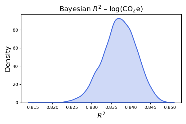
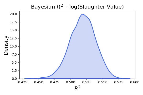
Finally the code for Bayesian R square plotting. See Gelman et al. (2019) for details.

## Compute R square

gamma_df=load_gamma_calib(num_sites, "reg")
theta_df=load_theta_calib(num_sites, "reg")


gamma_R2_draws = []
for s in range(len(sigma_u_gamma)):
    beta_s = beta_gamma[s, :]    # (K,)
    nu_s = nu_gamma[s, :]        # (B,)
    sigma_s = sigma_u_gamma[s]               # scalar

    yhat_s = gamma_df["X_gamma"] @ beta_s.T + nu_s[gamma_df["m_gamma"]-1]
    residual_s = np.array(gamma_df["y_gamma"]) - yhat_s

    var_fit = np.var(yhat_s, ddof=1)
    var_res = np.var(residual_s, ddof=1)

    
    # var_fit = np.var(yhat_s, ddof=1)
    # var_res = sigma_s ** 2

    R2 = var_fit / (var_fit + var_res)
    gamma_R2_draws.append(R2)

gamma_R2_draws = np.array(gamma_R2_draws)

print("Gamma Bayesian R^2 summary:")
print(f"Mean:   {np.mean(gamma_R2_draws):.4f}")
print(f"Median: {np.median(gamma_R2_draws):.4f}")
print(f"Std:    {np.std(gamma_R2_draws):.4f}")


plt.hist(gamma_R2_draws, bins=30, edgecolor='black',density=True)
plt.title(r"Bayesian $R^2$ - log(CO2e)", fontsize=16)
plt.xlabel("$R^2$", fontsize=16)
plt.ylabel("density", fontsize=16)
plt.savefig(get_path("output", "figures") / f"bayesian_r2_gamma_{num_sites}.png")
plt.close()




plt.figure(figsize=(6, 4))
sns.kdeplot(gamma_R2_draws, fill=True, color="royalblue", linewidth=2)
plt.title(r"Bayesian $R^2$ – log(CO$_2$e)", fontsize=16)
plt.xlabel("$R^2$", fontsize=16)
plt.ylabel("Density", fontsize=16)
plt.tight_layout()
plt.savefig(get_path("output", "figures") / f"kde_bayesian_r2_gamma_{num_sites}.png")
plt.close()



theta_R2_draws = []
for s in range(len(sigma_u_theta)):
    beta_s = beta_theta[s, :]    # (K_theta,)
    nu_s = nu_theta[s, :]        # (B_theta,)
    sigma_s = sigma_u_theta[s]   # scalar

    
    
    yhat_s = theta_df["X_theta"] @ beta_s.T + nu_s[theta_df["m_theta"] - 1]
    residual_s = np.array(theta_df["y_theta"]) - yhat_s

    var_fit = np.var(yhat_s, ddof=1)
    var_res = np.var(residual_s, ddof=1)

    


    R2 = var_fit / (var_fit + var_res)
    theta_R2_draws.append(R2)

theta_R2_draws = np.array(theta_R2_draws)

# Summary
print("Theta Bayesian R^2 summary:")
print(f"Mean:   {np.mean(theta_R2_draws):.4f}")
print(f"Median: {np.median(theta_R2_draws):.4f}")
print(f"Std:    {np.std(theta_R2_draws):.4f}")


# Plot
plt.hist(theta_R2_draws, bins=30, edgecolor='black',density=True)
plt.title(r"Bayesian $R^2$ - log(Slaughter Value)", fontsize=16)
plt.xlabel("$R^2$", fontsize=16)
plt.ylabel("density", fontsize=16)
plt.savefig(get_path("output", "figures") / f"bayesian_r2_theta_{num_sites}.png")
plt.close()


# Plot
plt.figure(figsize=(6, 4))
sns.kdeplot(theta_R2_draws, fill=True, color="royalblue", linewidth=2)
plt.title(r"Bayesian $R^2$ – log(Slaughter Value)", fontsize=16)
plt.xlabel("$R^2$", fontsize=16)
plt.ylabel("Density", fontsize=16)
plt.tight_layout()
plt.savefig(get_path("output", "figures") / f"kde_bayesian_r2_theta_{num_sites}.png")
plt.close()

---