Robust Inattentive Discrete Choice

Notebook written by Chun Hei Hung

This notebook describes the code used to solve the following problem described in Section 5 of the paper:

\[ \max_{p \in \Delta(A|X),q \in \Delta(A)} \min_{\mu \in \Delta(X)} \sum_x{ \mu(x) \left[ G(p,q)(x)+\xi \log{\frac{\mu(x)}{\hat{\mu}(x)}} \right] } \]

Where:

\[ G(p,q)(x) = \sum_a{p(a|x)\left[u(x,a)-\lambda \log{\frac{p(a|x)}{q(a)}}\right]} \]

Using the numerical algorithm from Section 3. It is divided into two sections: the first section applies the algorithm for a given set of \((\alpha,\lambda,\xi)\), while the second section constrains the information by \(\kappa\) and calculates the optimal \(\lambda\) for a given set \((\alpha,\xi)\).

1 Base Case

1.1 Solution Code Overview

The function solve implements the numerical algorithm for a given set of parameters, and outputs the solution and related objects of interest.

First, the user should specify the values of \(\alpha,\lambda,\xi\) over which solve should be evaluated. Each of these are arrays of type float. Each array can have different lengths.

Array	Domain restrictions	Description	Default
alpha_array	0 to 1	Coefficient of risk aversion, where \(\alpha=0\) is the linear utility and values close to \(1\) approximate the log utility case	10 evenly spaced points from 0 to 0.9
Lam_array	Greater or equal to 1 (less than 1 causes convergence issues)	Information cost, where large values, e.g. \(\mathbb{I}=100\), approximate zero information cost	[10.0]
xi_array	Greater or equal to 1	Robustness parameter, where large values, e.g. \(\mathbb{R}=100\), approximate no robustness adjustment	10 evenly spaced points from 1 to 100

Second, the user should specify the following parameters:

Input	Type	Description	Default
N	int	Number of states	2
M	int	Number of actions	3
hat_mu	\(N \times 1\) ndarray	Baseline prior: does not affect the solution in this model	Uniform prior
eps	float	Tolerance: the higher the tolerance, the more accurate the solution but the longer the computation time. Tolerance of \(10^{-6}\) or lower is recommended as a baseline	\(10^{-6}\)
q_step,p_step,mu_step	float	Step-size: for each variable \(x \in \{p,q,\mu\}\) in the algorithm. The larger the step-size, the greater the adjustment from \(x_t\) to \(x_{t+1}\), with 1 meaning full adjustment. A larger step-size reduces the occurrence of convergence issues but increases computation time. Step-size of \(0.1\) will ensure convergence for the parameters described in the paper	\(0.1\)
payoff_set	\(M \times N\) ndarray	Payoff matrix: the dimensions of this input must be \((M,N)\). If the user wishes to use the payoff matrix specified in the paper parameterized by \(r\), they can simply change \(r\) without changing the payoff matrix	\([[0,2r],[r,0],[5,5]]\)

solve generates the following outputs:

Output	Type	Description	Notation in manuscript
objective	float	Optimal value of objective function	\(\mathbb{E}[u(x,a)] - \lambda \mathbb{I} + \xi \mathbb{R}\) given \((p^*,q^*,\mu^*)\)
p	\(M \times N\) ndarray	State-dependent decision rule: entry \((i,j)\) of this array corresponds to the probability of choosing action \(i\) given state \(j\)	\(p^*(a|x)\)
q	\(M \times 1\) ndarray	Worst-case marginal distribution over actions	\(q^*(a)\)
mu	\(N \times 1\) ndarray	Worst-case prior	\(\mu^*\)
information	float	Optimal value of mutual information	\(\mathbb{I}(p^*,q^*)\)
entropy	float	Optimal value of relative entropy	\(\mathbb{R}(\mu^*,\hat{\mu})\)

1.2 Quick Start

Let’s start by importing the necessary Python libraries and functions.

#If using Google Colab, run the following code. Otherwise, ignore:
!git clone https://github.com/lphansen/rational_inattention
import os
os.chdir("rational_inattention/sphinx")

import numpy as np
import matplotlib.pyplot as plt
import os
import pickle
from src import solve, plot, save_results

Next, we can specify the \((\alpha,\lambda,\xi)\) grid:

#Arrays
alpha_array = np.linspace(0.0,0.9, 10)
Lam_array = [10.0]
xi_array = np.linspace(1.0, 100.0, 10)

A, L, X = np.meshgrid(alpha_array, Lam_array, xi_array, indexing='ij')

#Initialize grid of results
results = np.zeros((len(alpha_array), len(Lam_array), len(xi_array)), dtype=object) 

Finally, we specify the parameters:

#Parameters
N = 2  # Number of states
M = 3  # Number of actions
r = 7.5 # Parameterization of the payoff set
payoff_set = np.array([[0.0, r * 2], [r, 0.0], [5.0, 5.0]]) # If you want to use the payoff matrix in the paper, do not change this variable; instead, change r
eps = 1e-6  # Error tolerance

# Time-step increments
q_step = 0.1
p_step = 0.1
mu_step = 0.1

# Baseline prior
hat_mu = np.ones(N)*(1/N) # Uniform prior 

# Check that payoff matrix is correctly specified
if payoff_set.shape != (M, N):
    raise ValueError("Payoff set must be of shape (M, N)")

# Collect parameters
params = [M, N, hat_mu, eps, q_step, p_step, mu_step,payoff_set]

Now we run solve at each point in our \(\alpha,\lambda,\xi\) grid. Under the default settings, this takes 40 seconds.

for alpha in range(len(alpha_array)):
    for lam in range(len(Lam_array)):
        for xi in range(len(xi_array)):
            results[alpha,lam,xi] = solve(X[alpha,lam,xi], L[alpha,lam,xi], A[alpha,lam,xi], params)

The user can save the results as a pkl file with name specified by results_name using the following code.

results_name = 'experiment1'
save_results(results_name, results, alpha_array, Lam_array, xi_array, params)

1.3 Plotting

The user can plot the results along a chosen axis, holding the other two axes fixed, using the code below.

Specifying axis as 0 will plot the results with \(\alpha\) on the \(x\) axis; 1 will plot \(\lambda\); and 2 will plot \(\xi\). The other two variables will be fixed at the indices specified by fixed_values. For example, the default settings below plot the results with \(\xi\) on the \(x\) axis, with \(\alpha\) and \(\lambda\) fixed at the first entry of their respective arrays. The plot will automatically be saved in the plots folder under plot_name, which can be specified below.

axis = 2
fixed_values = [0,0]
plot_name = 'plot1'
plot(results, alpha_array, Lam_array, xi_array, axis, fixed_values,plot_name)

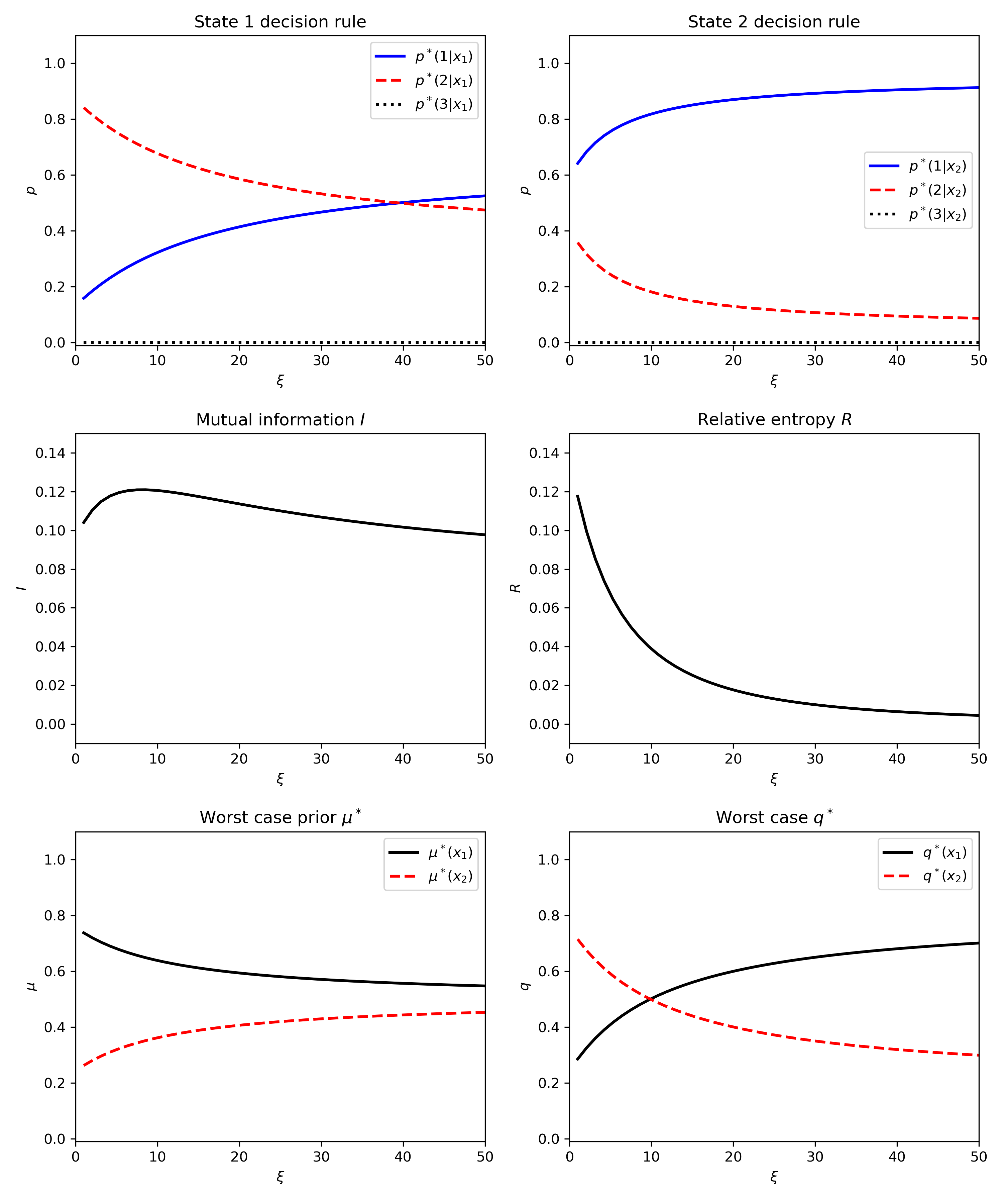
Fig. 1 Example figure taken from Figure 2 of the paper.

2 Mutual Information Constraint

2.1 Solution Code Overview

In the following section, we constrain mutual information and allow \(\lambda\) to vary to satisfy this constraint:

\[ \mathbb{I}(p,q) \leq \kappa \]

To find the optimal \(\lambda\), we perform a grid search over Lam_grid and find the \(\lambda\) which maximises the objective while satisfying the above constraint. This is carried out by the function find_min_Lam. Therefore instead of defining Lam_array, we define the values of kappa for which we want to find a solution and solve for the implied_lambda.

Input	Type	Description	Default
kappa_array	ndarray	Array of constraints on mutual information	\([0.04]\)
Lam_grid	ndarray	Gridpoints of \(\lambda\): this must be sufficiently large to ensure accuracy	100 evenly spaced points between 1 and 10

2.2 Quick Start

First, define the new parameters:

from src import find_min_Lam
kappa_array = np.array([0.04])
Lam_grid = np.linspace(1.0, 10.0, 100)

We also need to define all the previous parameters.

#Arrays
alpha_array = np.linspace(0.0,0.9, 10)
xi_array = np.linspace(1.0, 100.0, 10)

A, K, X = np.meshgrid(alpha_array, kappa_array, xi_array, indexing='ij')

#Initialize grid of results
results = np.zeros((len(alpha_array), len(kappa_array), len(xi_array)), dtype=object) 
implied_lambda = np.zeros((len(alpha_array), len(kappa_array), len(xi_array)), dtype=float) 

#Parameters
N = 2  # Number of states
M = 3  # Number of actions
r = 7.5 # Parameterization of the payoff set
payoff_set = np.array([[0.0, r * 2], [r, 0.0], [5.0, 5.0]]) # If you want to use the payoff matrix in the paper, do not change this variable; instead, change r
eps = 1e-6  # Error tolerance

# Time-step increments
q_step = 0.1
p_step = 0.1
mu_step = 0.1

# Baseline prior
hat_mu = np.ones(N)*(1/N) # Uniform prior 

# Check that payoff matrix is correctly specified
if payoff_set.shape != (M, N):
    raise ValueError("Payoff set must be of shape (M, N)")

# Collect parameters
params = [M, N, hat_mu, eps, q_step, p_step, mu_step,payoff_set]

Next, we run find_min_Lam on our \(\lambda\) grid.

for alpha in range(len(alpha_array)):
    for kappa in range(len(kappa_array)):
        for xi in range(len(xi_array)):
            implied_lambda[alpha,kappa,xi] = find_min_Lam(A[alpha,kappa,xi], K[alpha,kappa,xi], X[alpha,kappa,xi], params,Lam_grid)
            if implied_lambda[alpha,kappa,xi] == None:
                results[alpha,kappa,xi] = None
                results[alpha,kappa,xi]['implied_lambda'] = None
            else:
                results[alpha,kappa,xi] = solve(X[alpha,kappa,xi], implied_lambda[alpha,kappa,xi], A[alpha,kappa,xi], params)
                results[alpha,kappa,xi]['implied_lambda'] = implied_lambda[alpha,kappa,xi]

2.3 Plotting

As before, we can use the plot function to visualize the solution:

axis = 2
fixed_values = [0,0]
plot_name = 'plot2'
plot(results, alpha_array, Lam_array, xi_array, axis, fixed_values,plot_name)

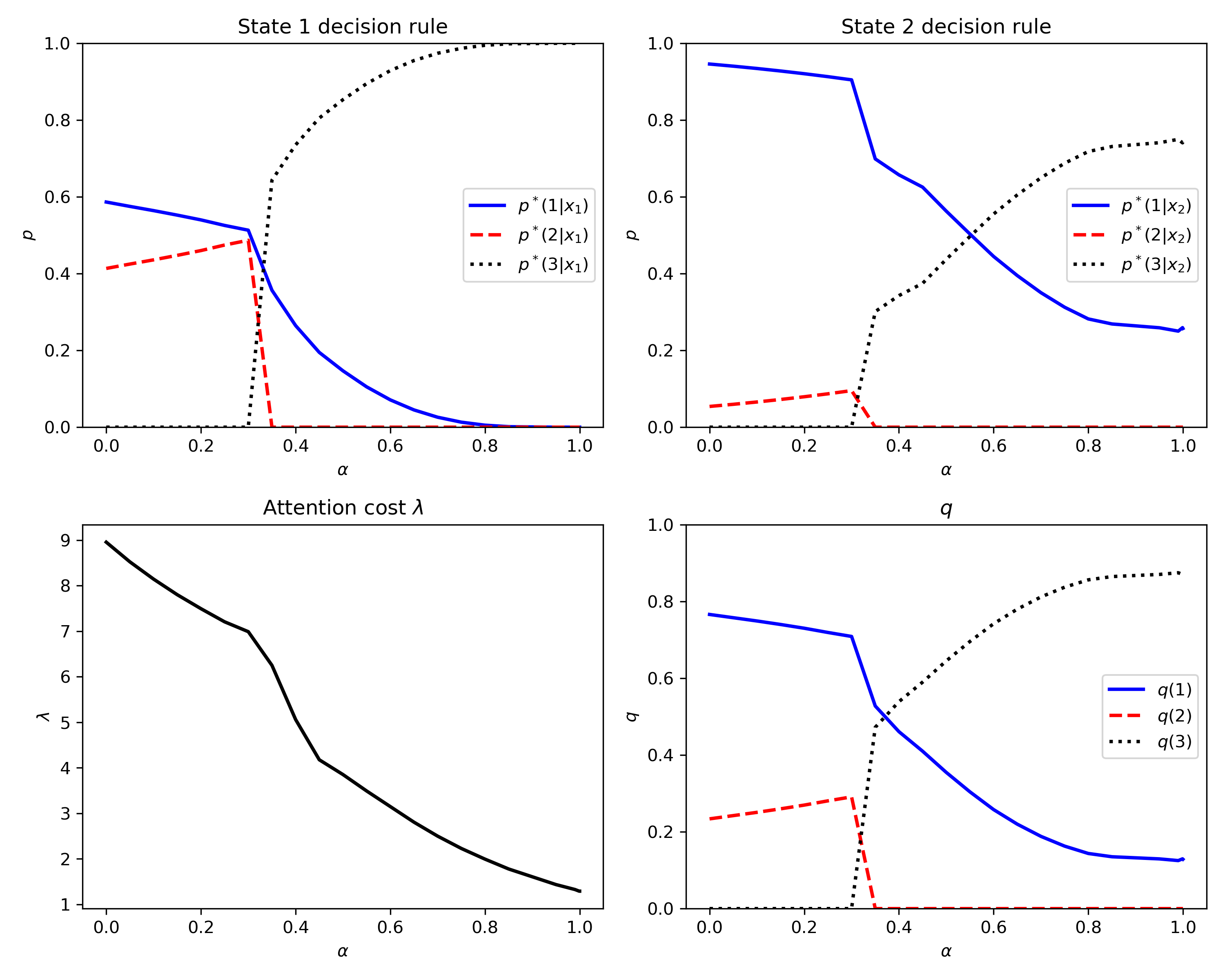
Fig. 2 Example figure taken from Figure 4 of the paper.